Color Palette Choice and Customization in R and ggplot2
Workshops for Ukraine
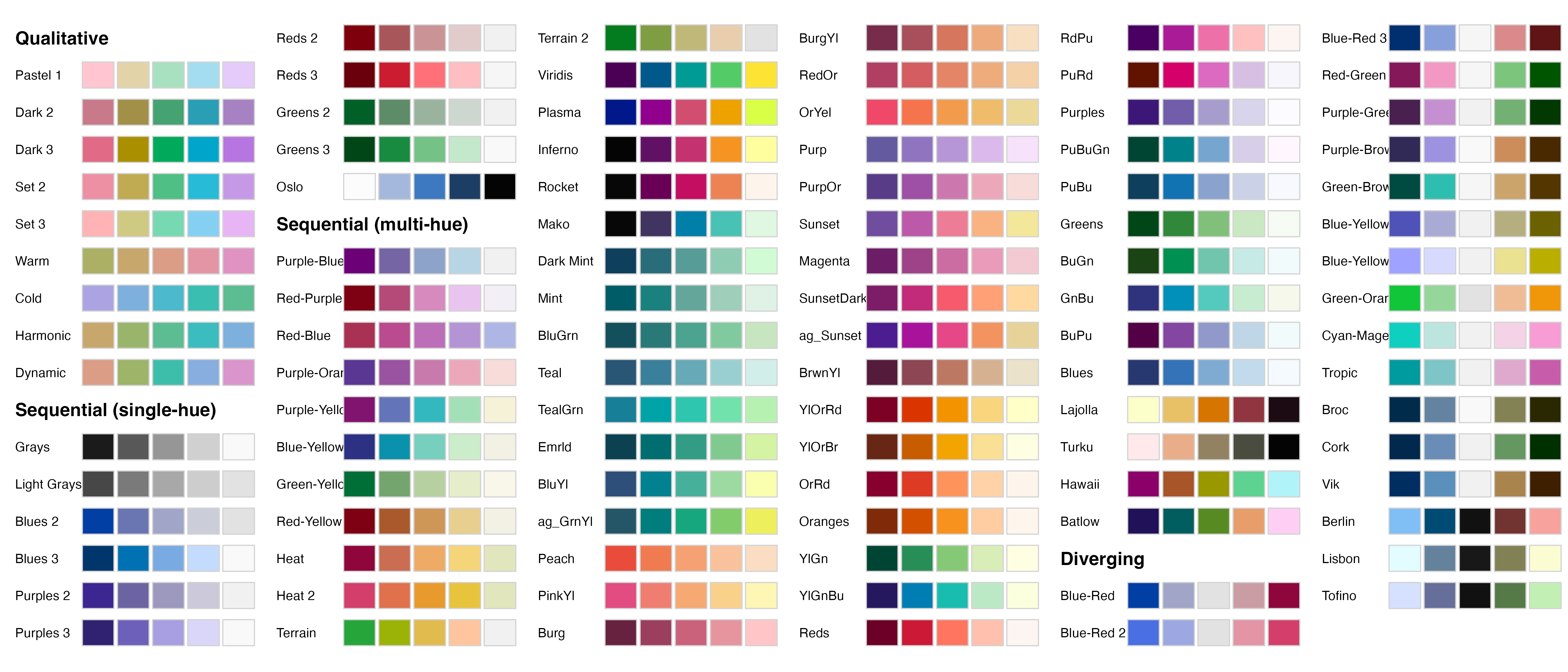
Color Definitions

Color Definitions


Color Definitions
Color Definitions
Demonstrate Colors
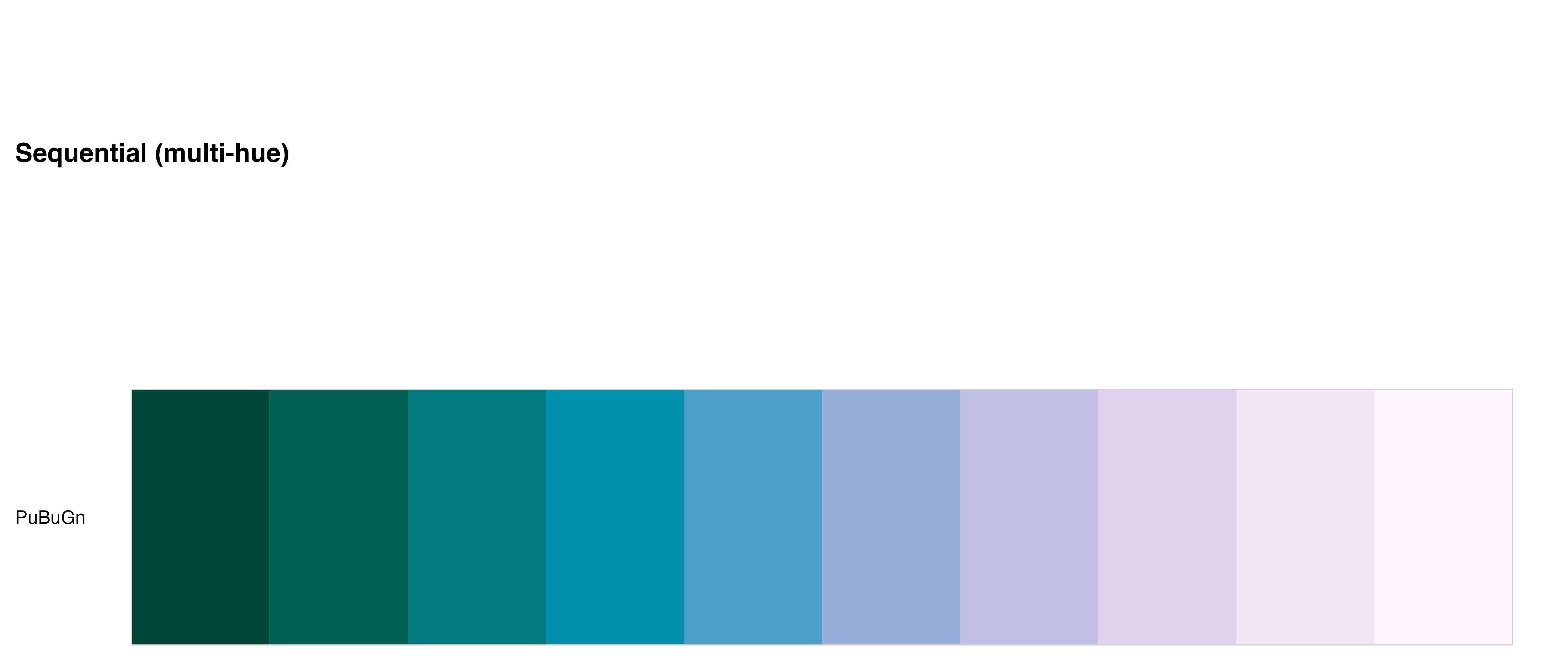
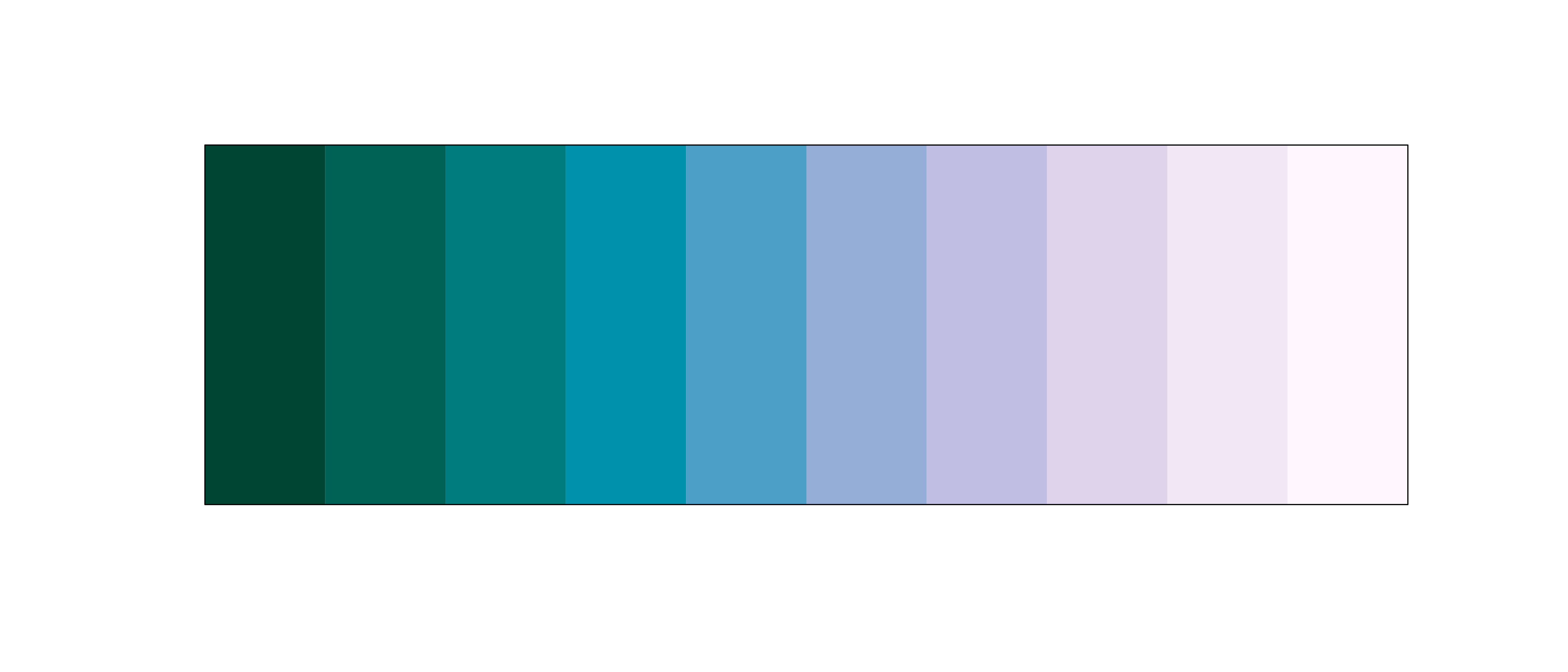
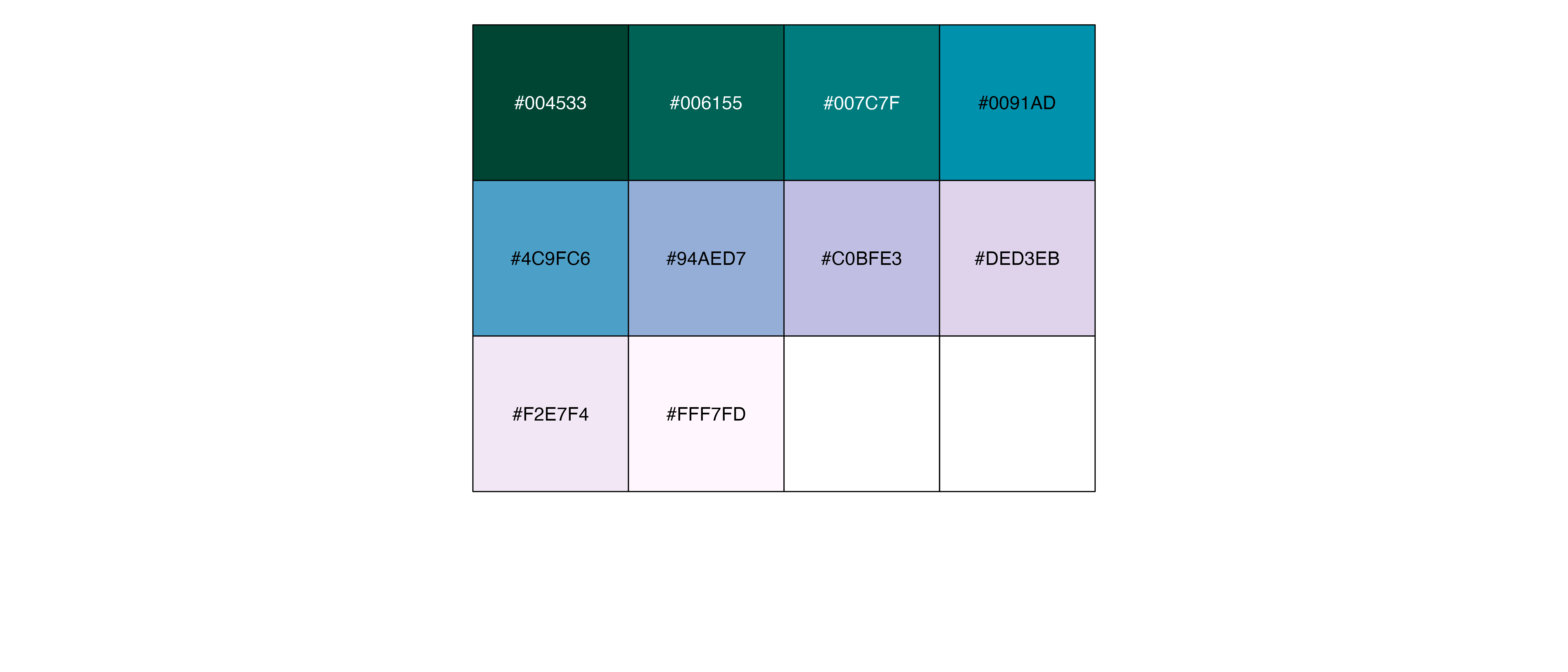
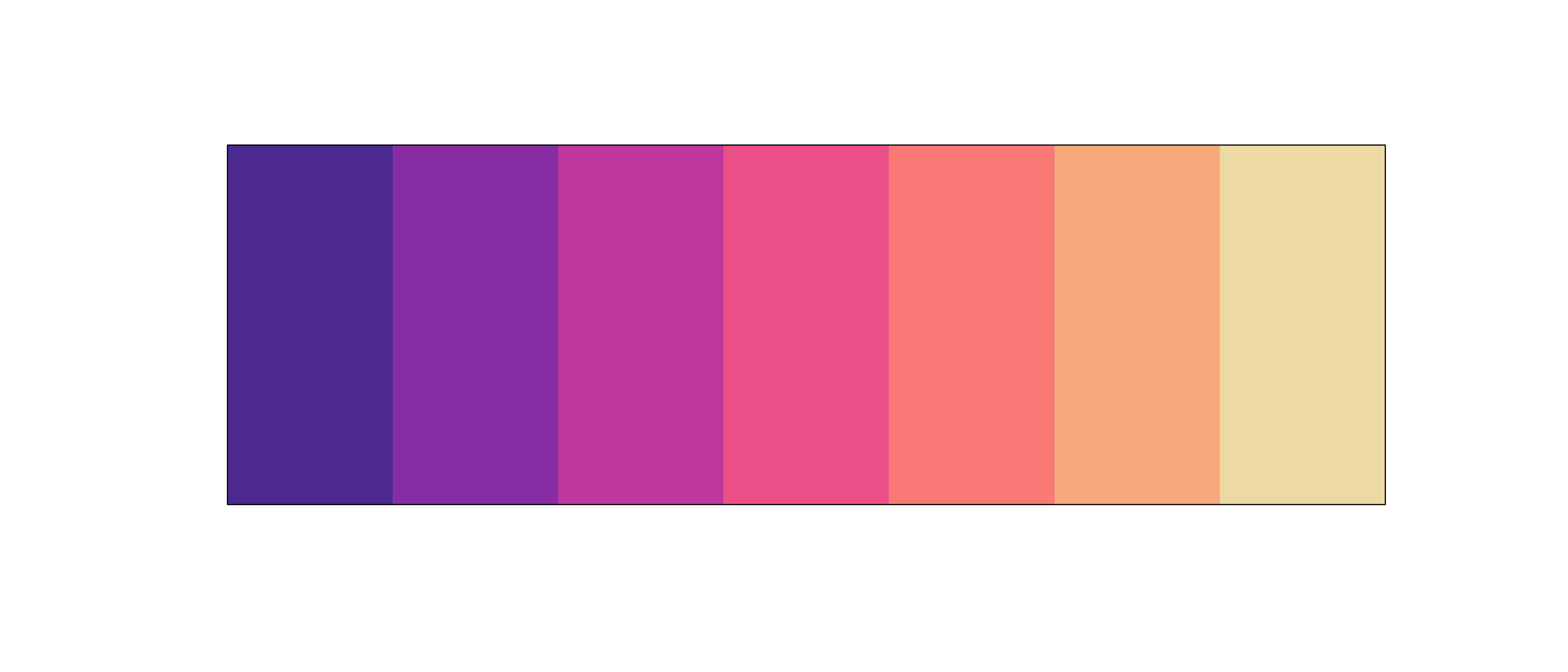
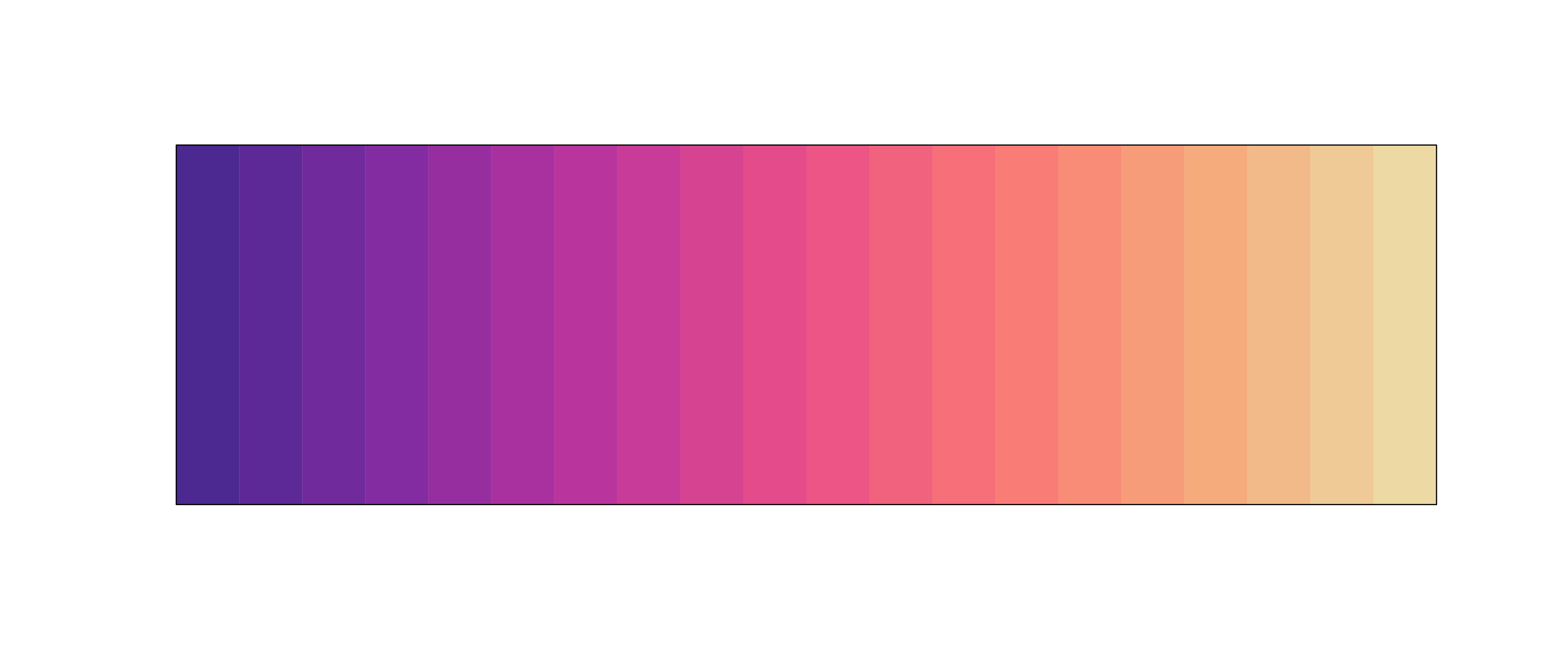
Create Sequential Color Palettes
Create Sequential Color Palettes
Create Sequential Color Palettes
Create Diverging Color Palettes

Create Diverging Color Palettes

Adjust Colors
Adjust Colors

Adjust Colors

Adjust Colors
Adjust Colors

Adjust Colors

Adjust Colors

Adjust Colors

Mix Colors

{colorspace}
{colorspace}
{colorspace}
{colorspace}
{RColorBrewer}
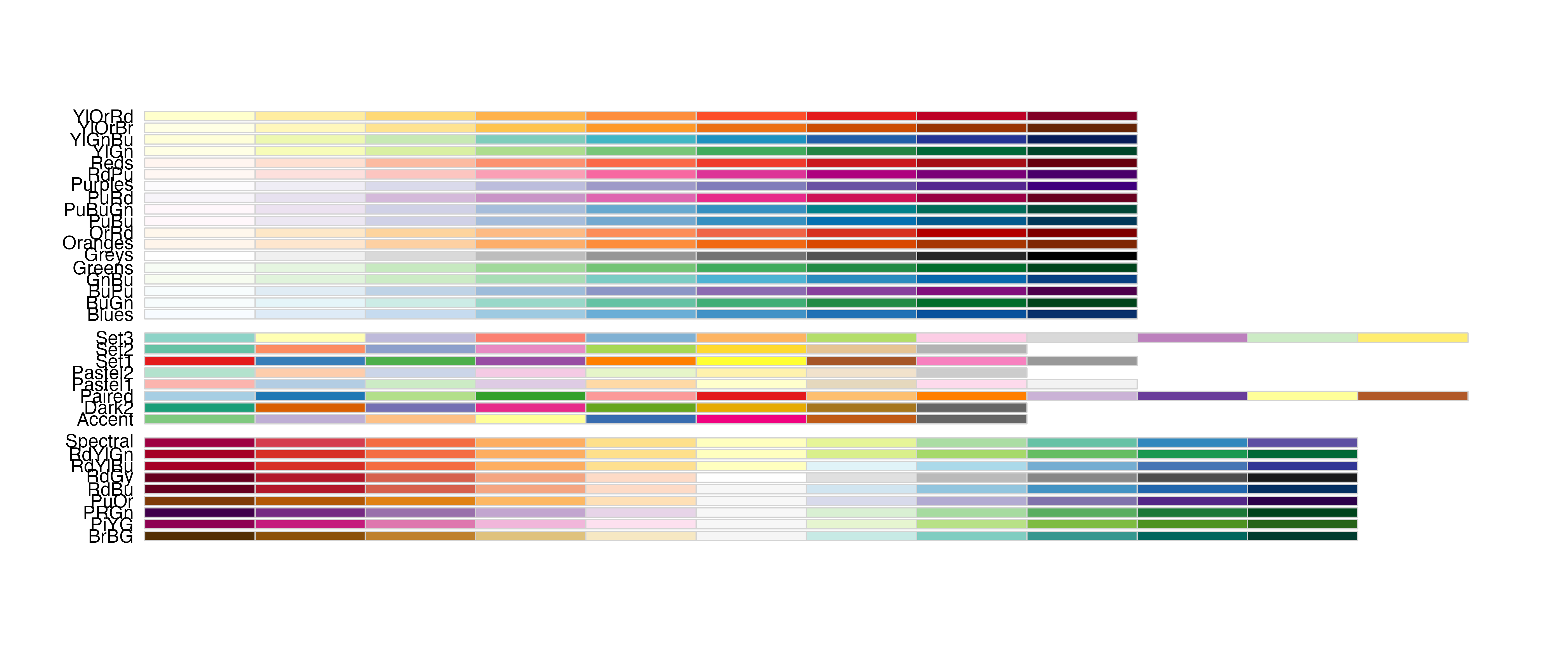
{RColorBrewer}
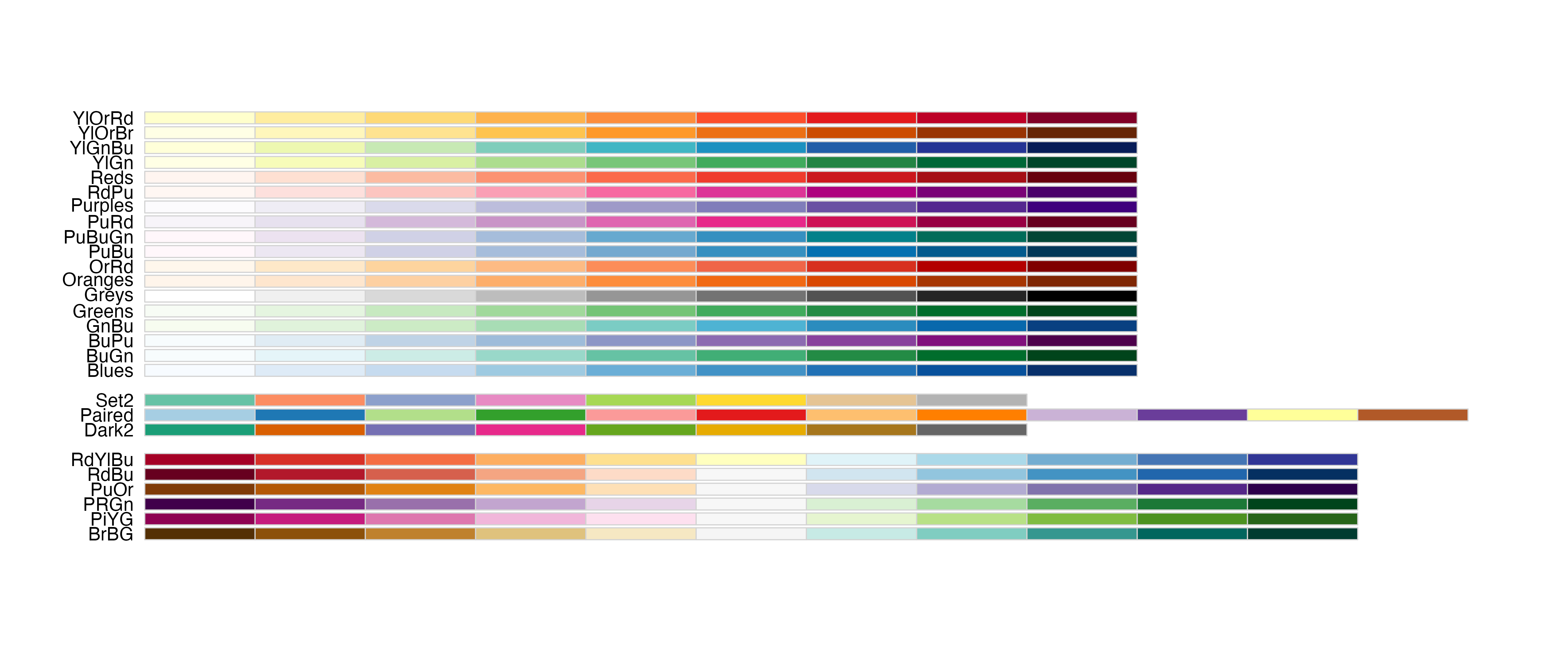
{RColorBrewer}

{scico}
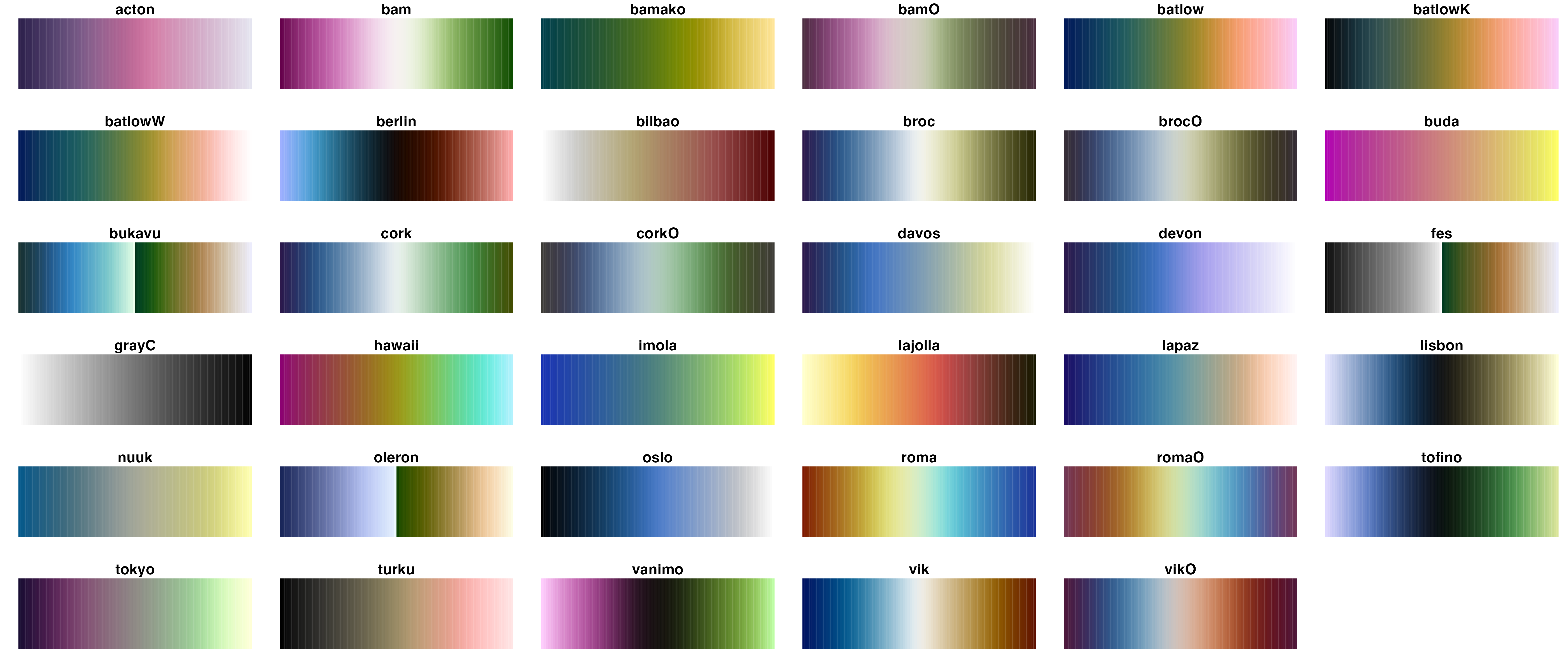
{scico}
{rcartocolor}
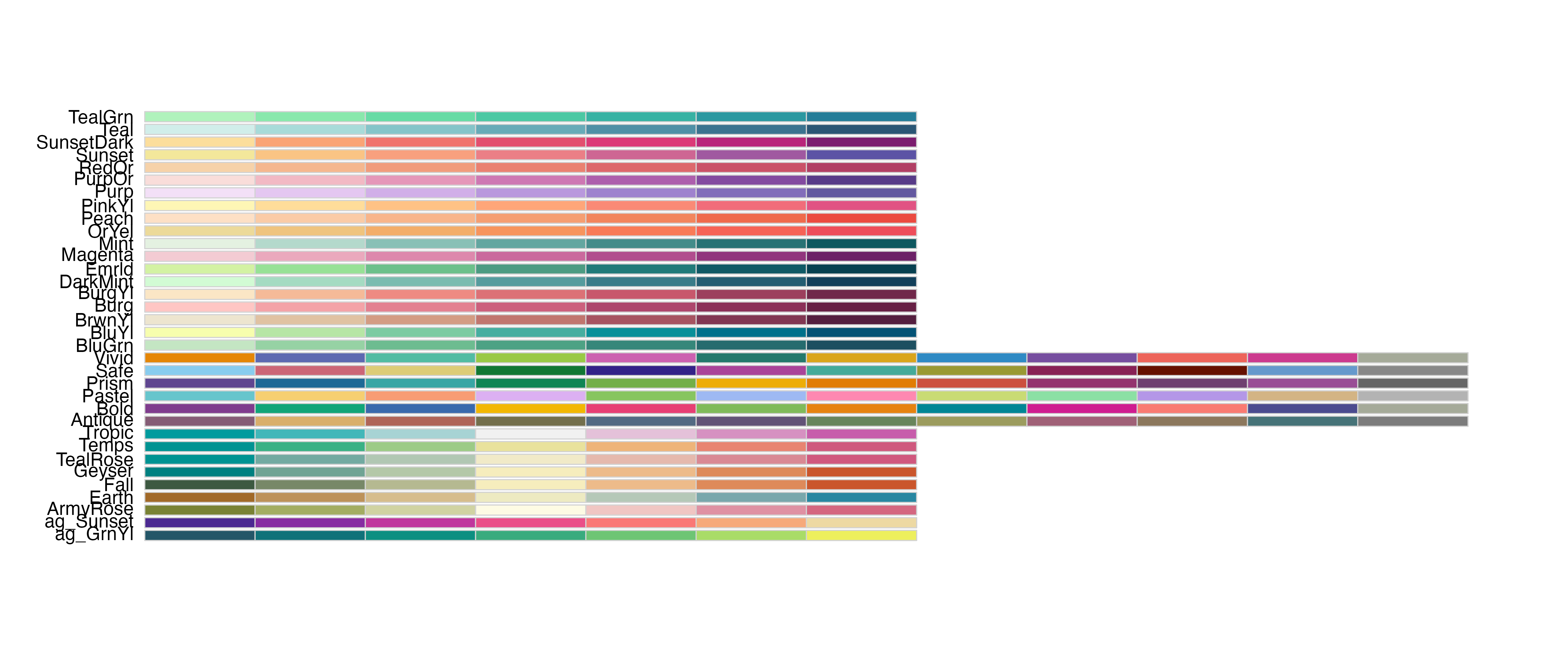
{rcartocolor}
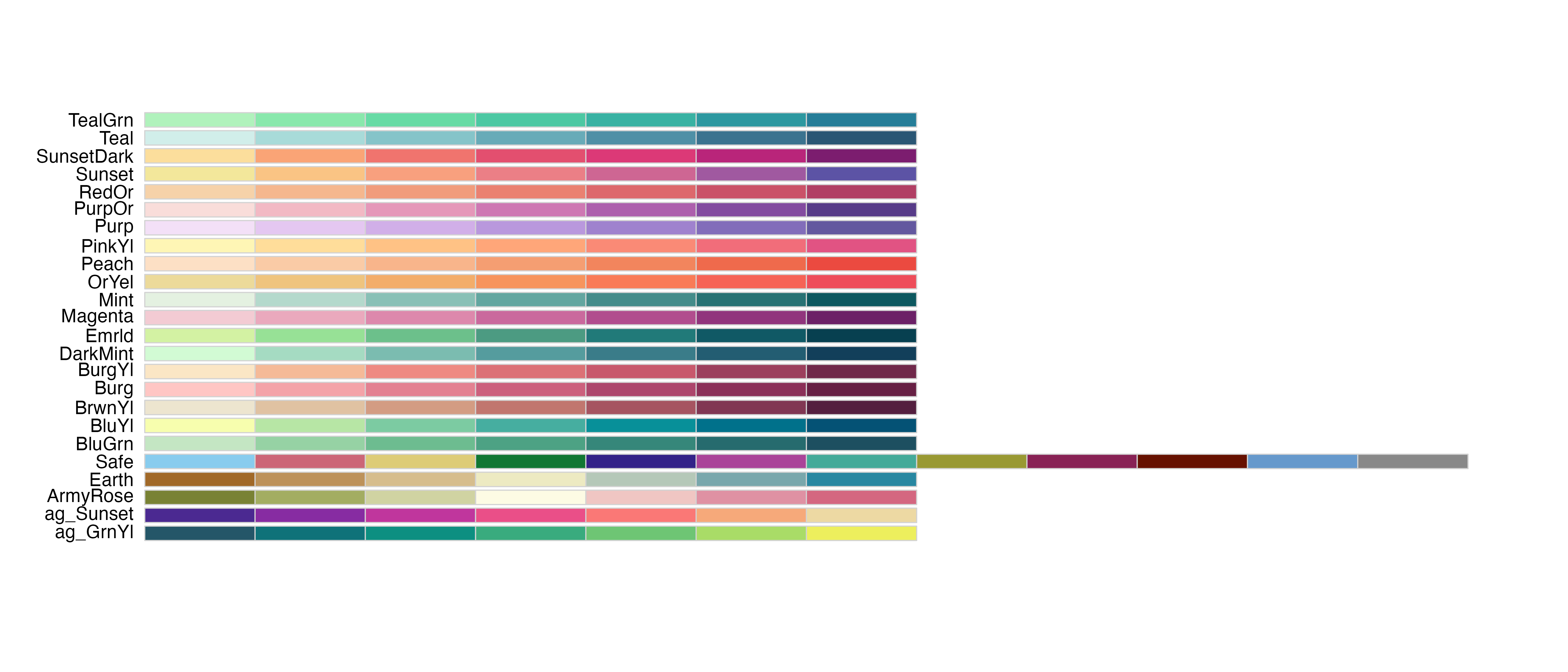
{rcartocolor}
{rcartocolor}
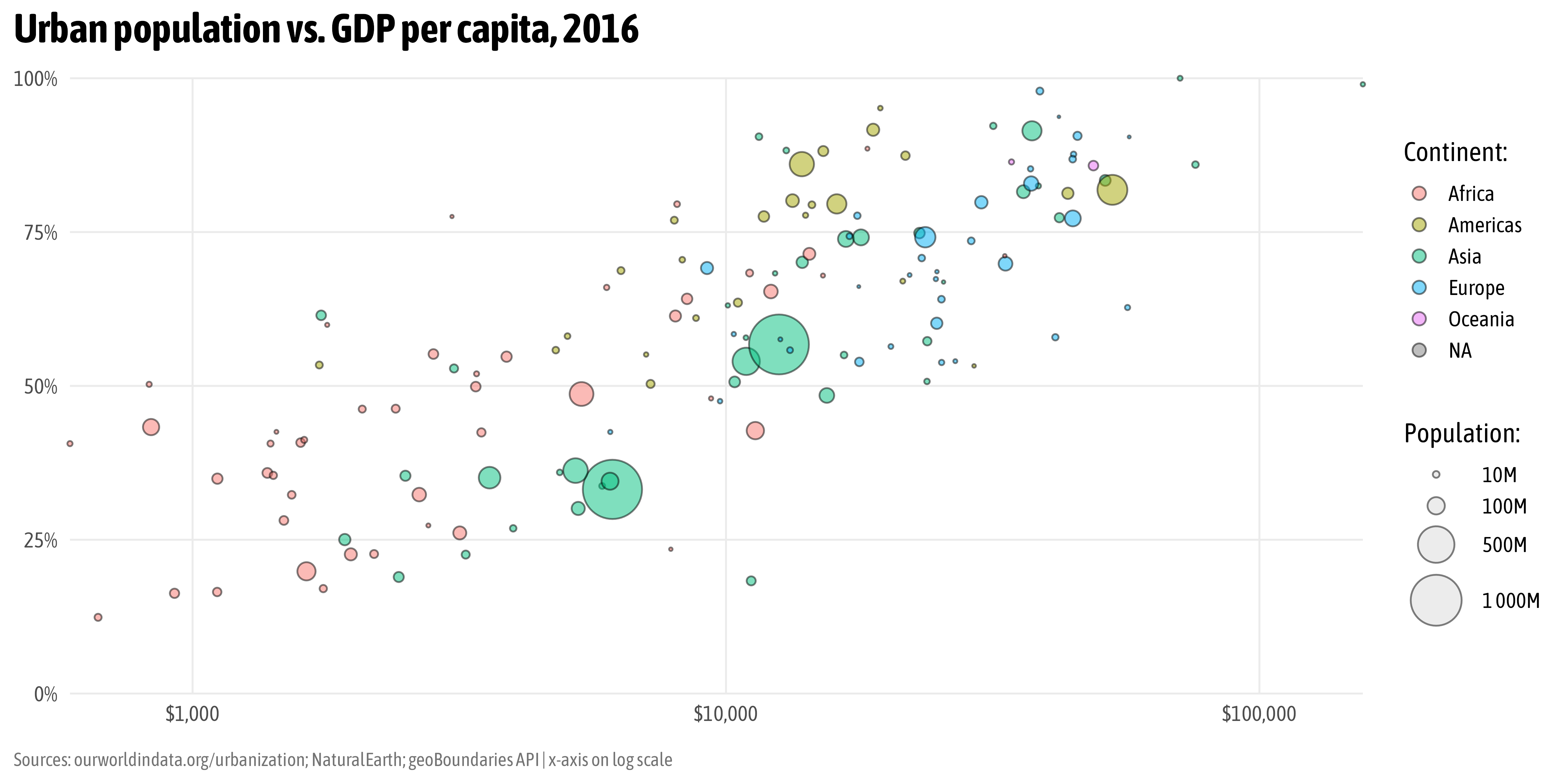
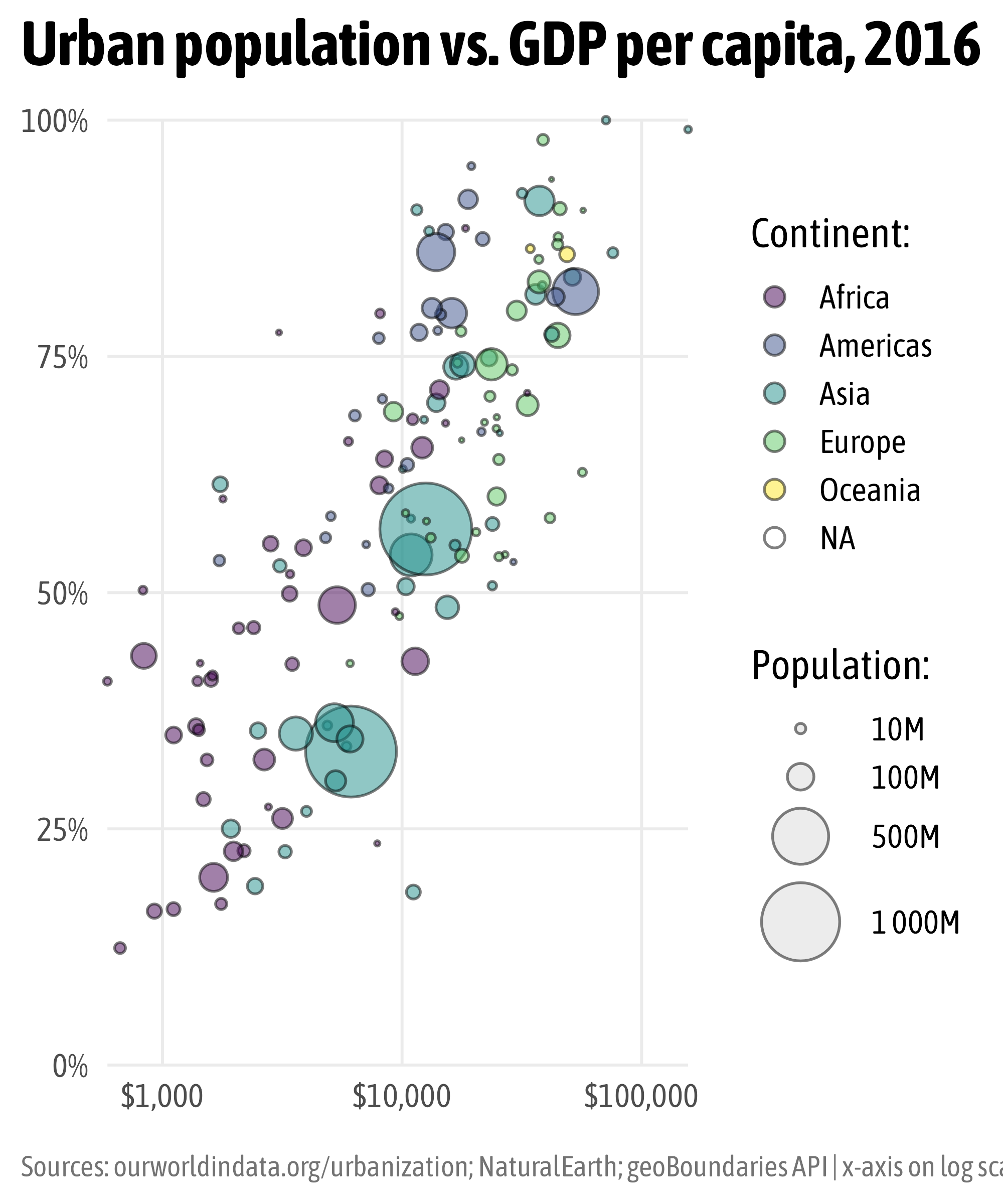
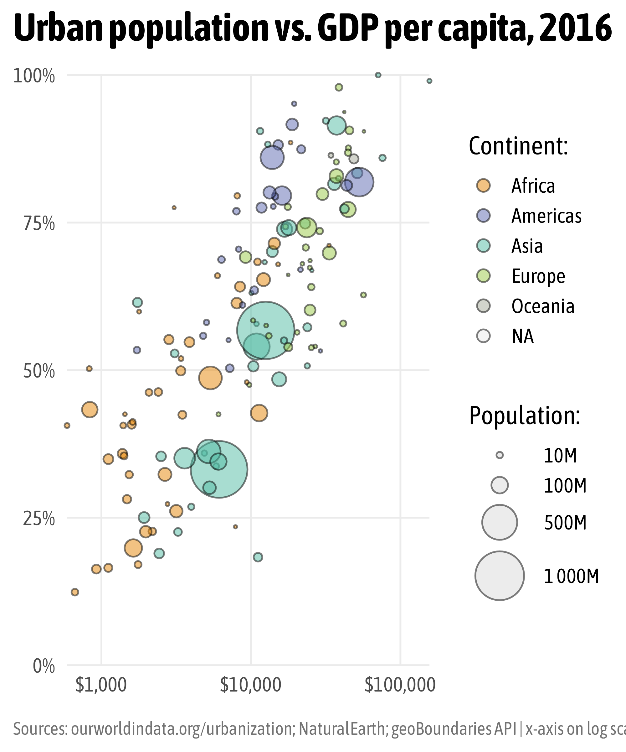
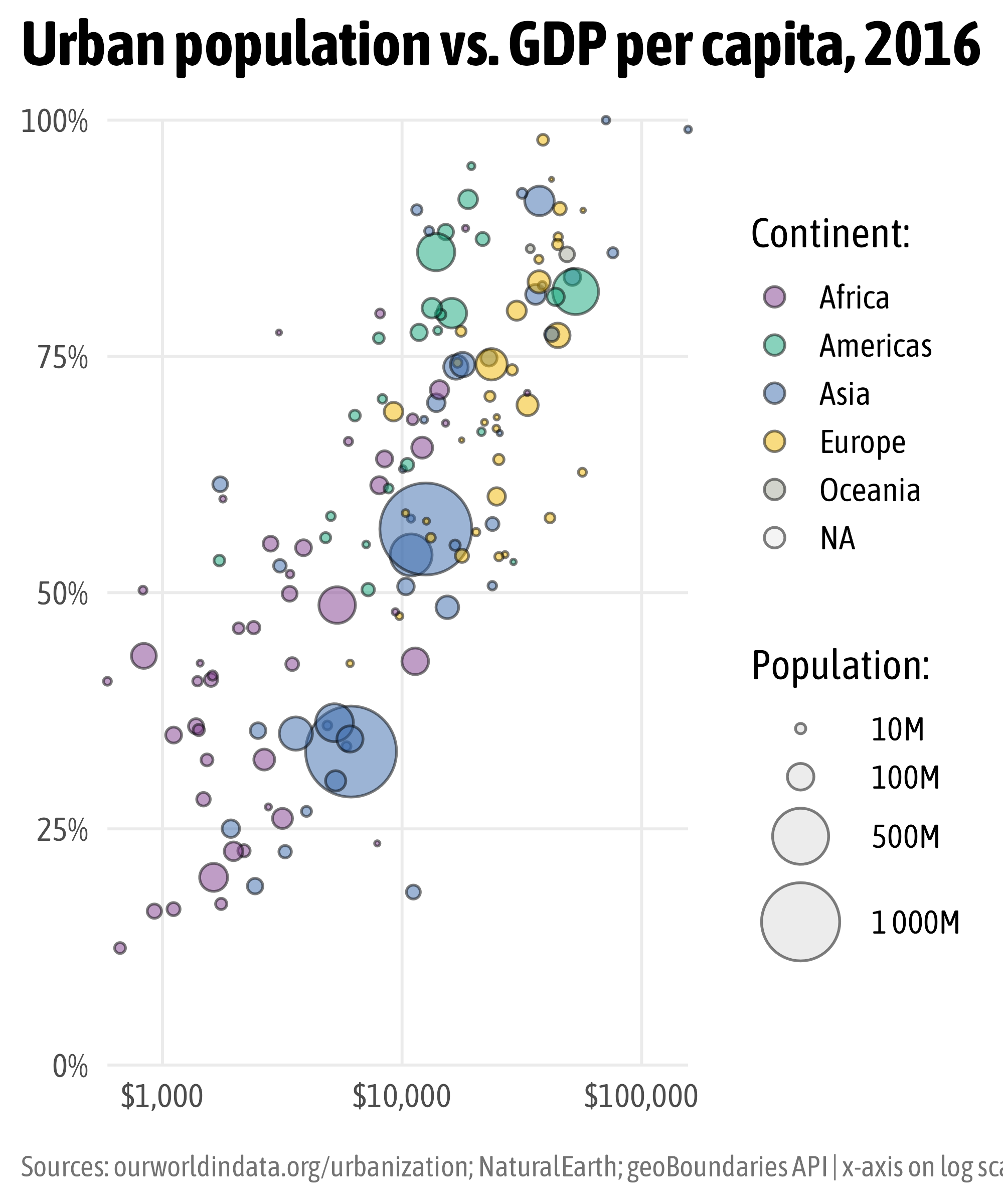
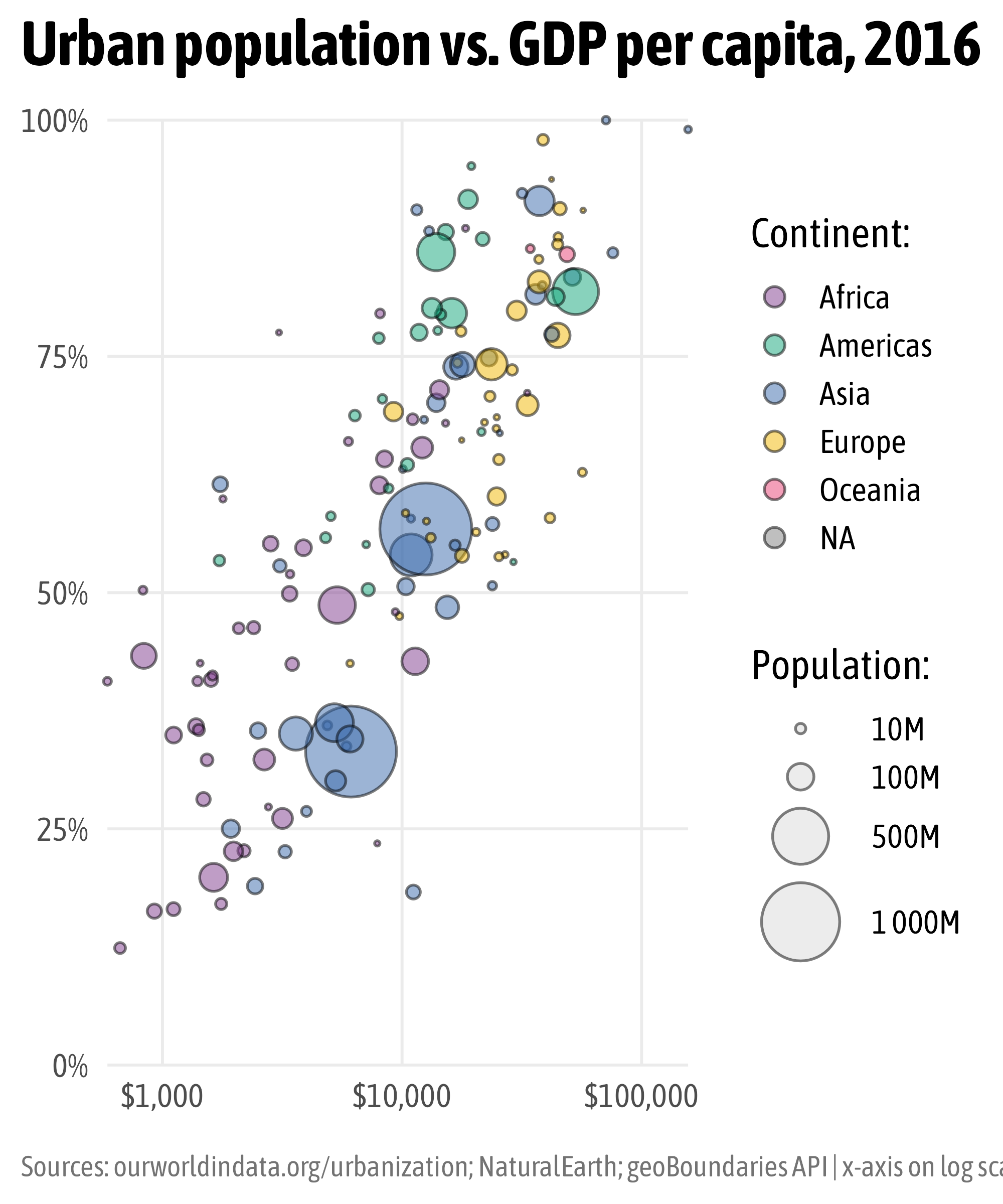
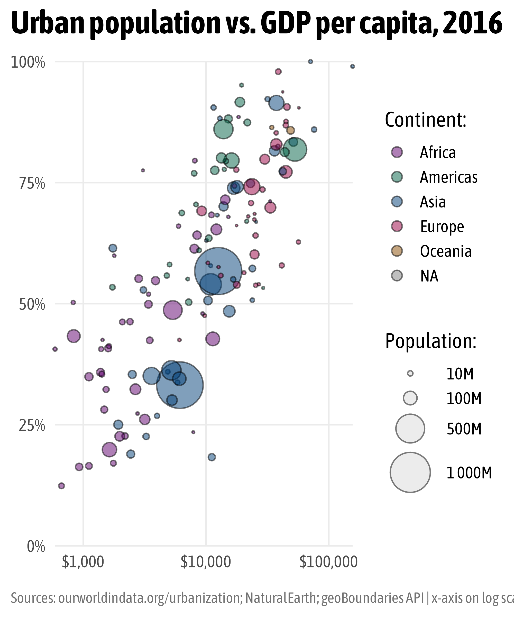
The Chart
{viridis}
{viridis}
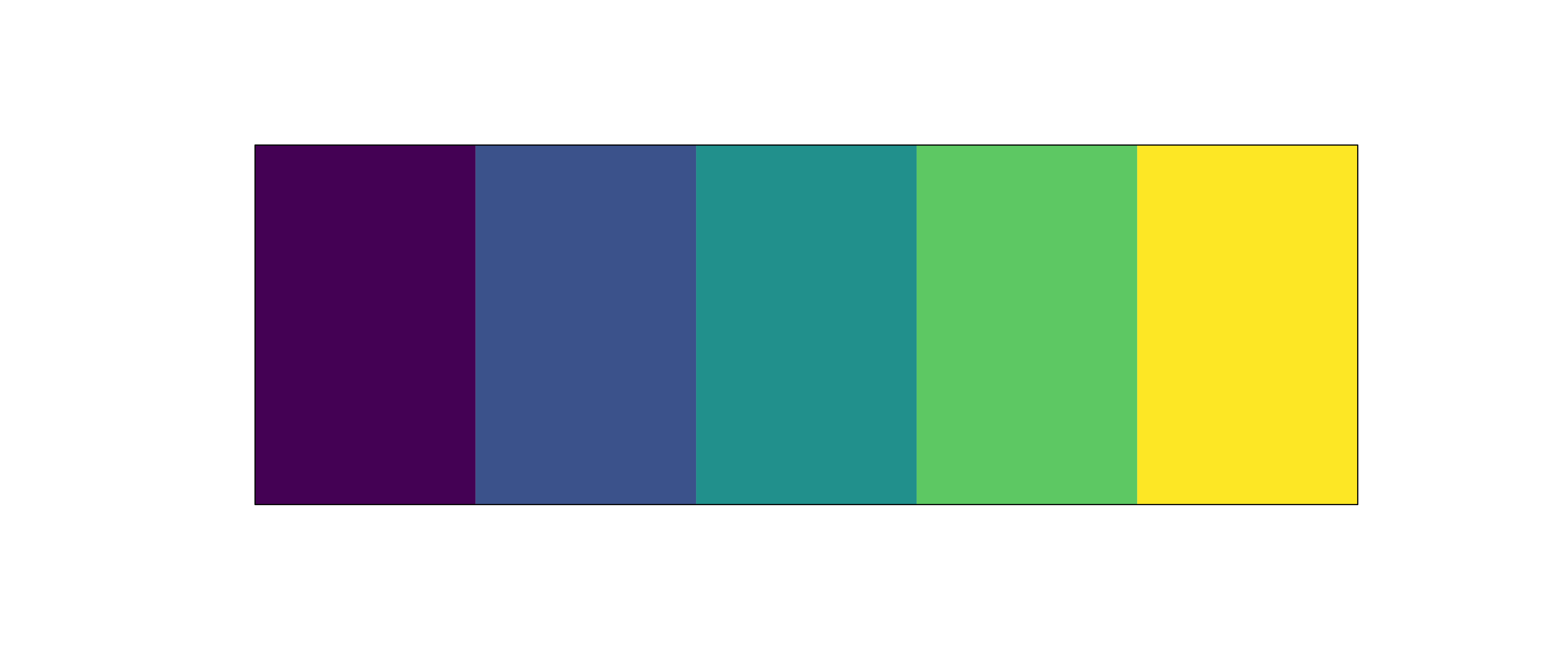
{viridis}
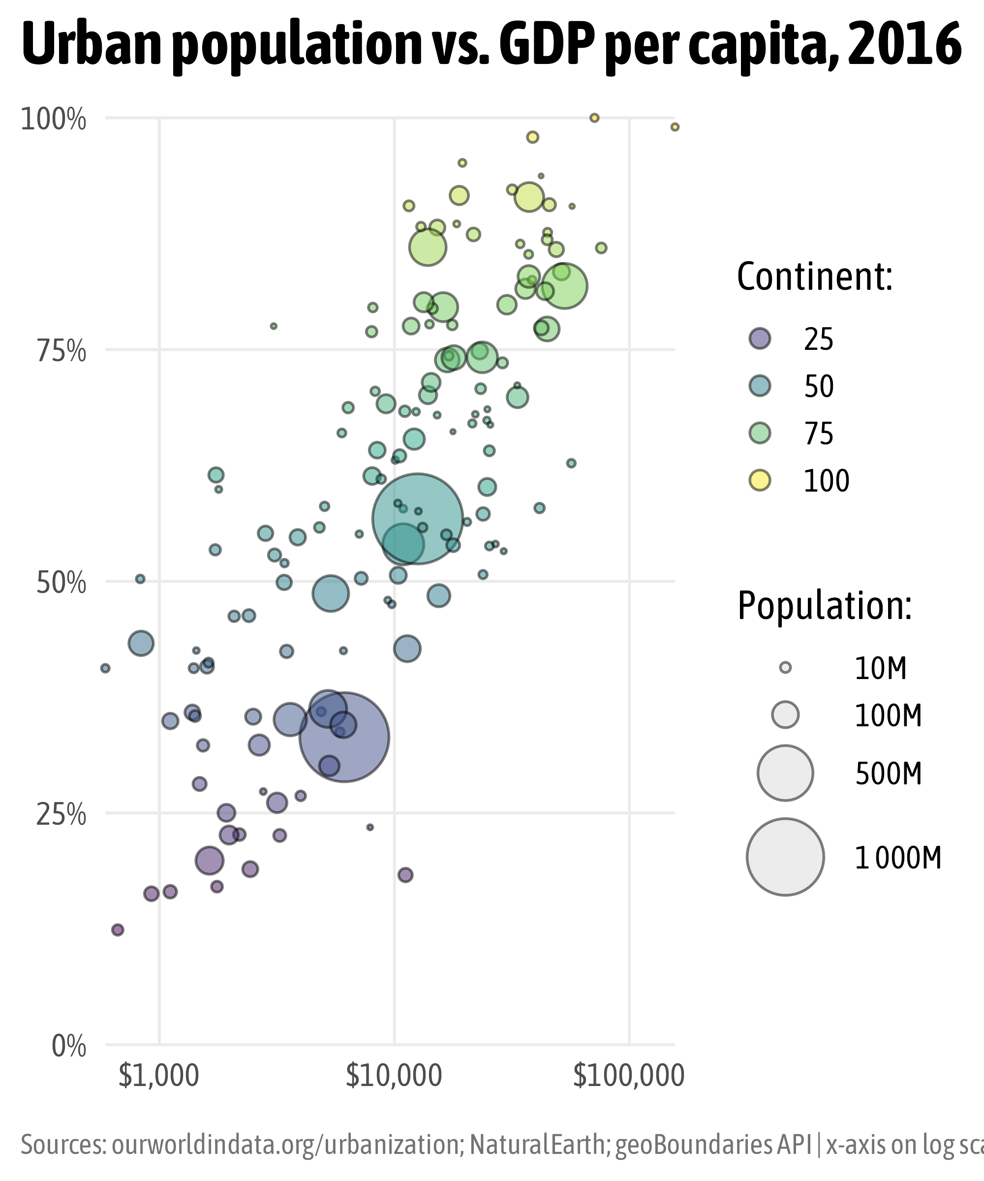
{viridis}
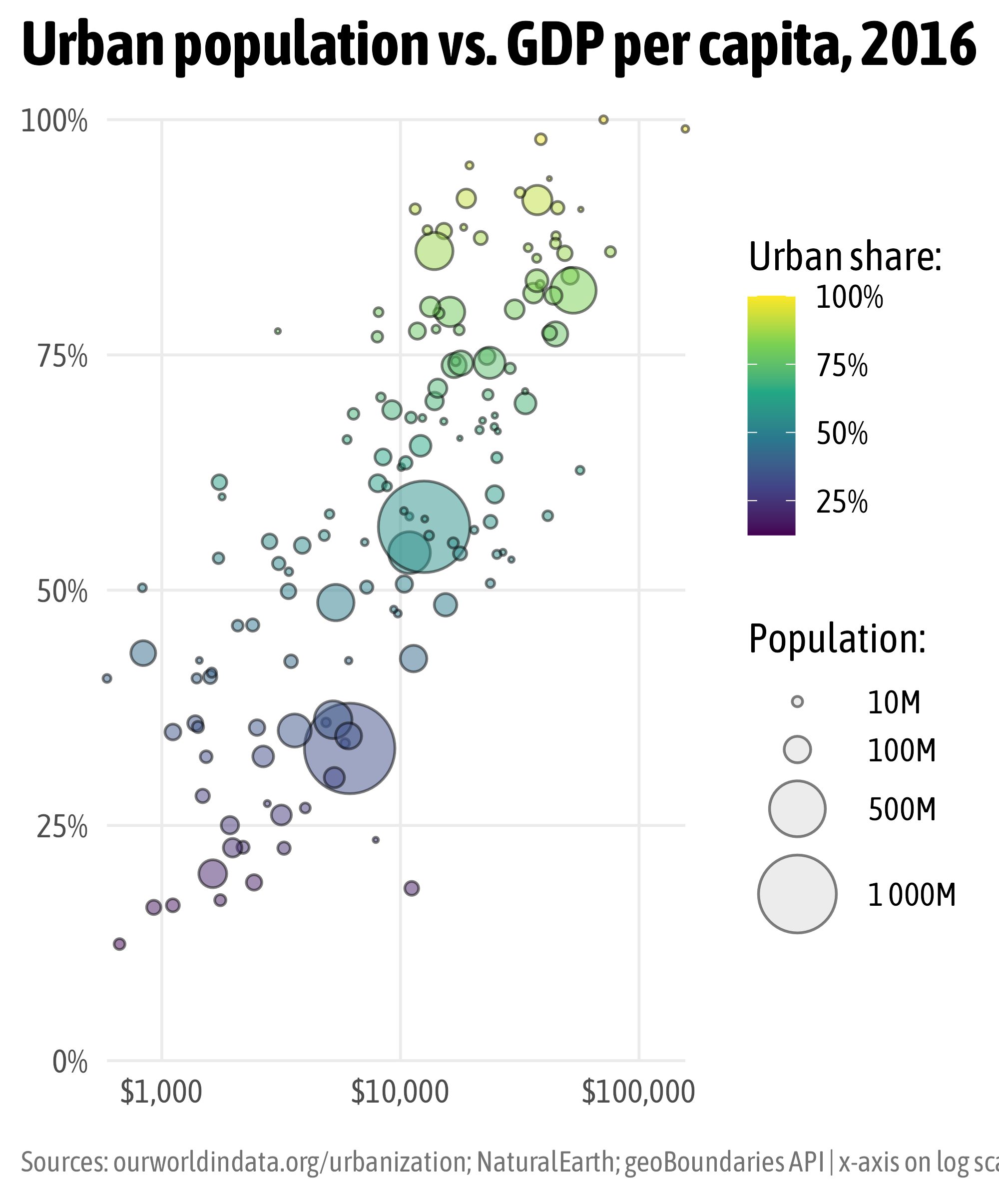
{rcartocolor}
{rcartocolor}
{rcartocolor}
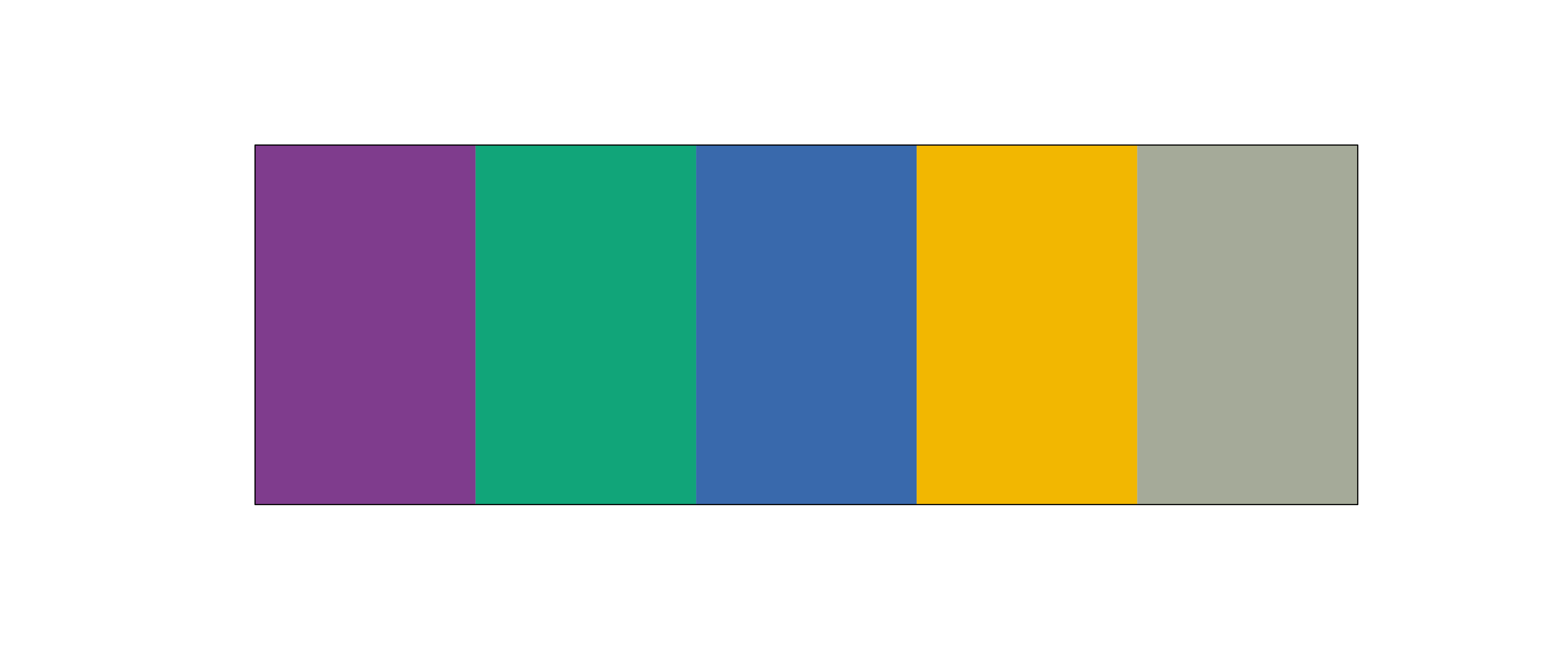
scale_color|fill_manual()

Customize Palette
Customize Palette

Customize Palette
Re-use Palettes
Re-use Palettes
Re-use Palettes
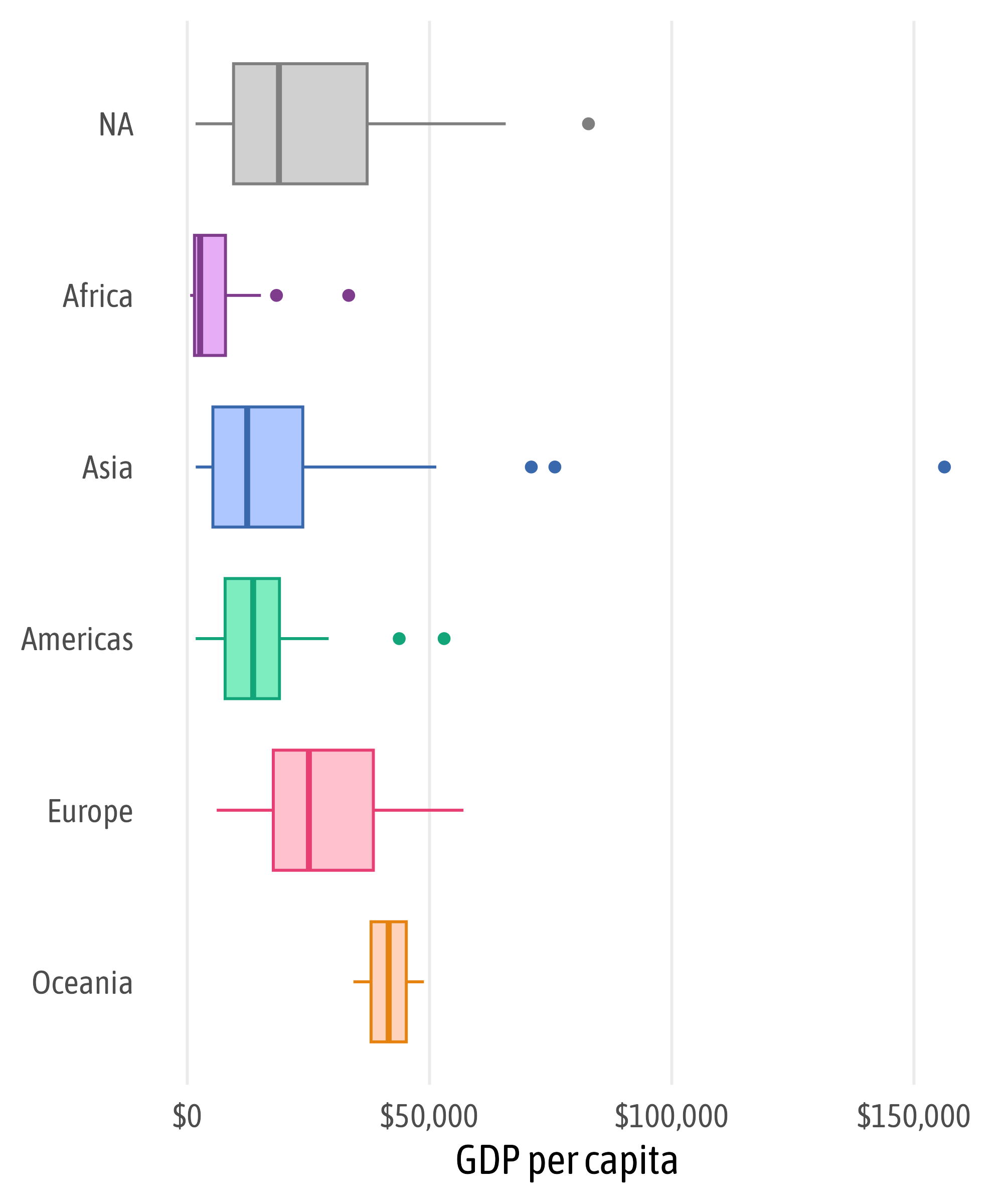
b <- ggplot(
    data = df_world,
    mapping = aes(
      x = gdp_per_capita,
      y = forcats::fct_reorder(
        region_un, -gdp_per_capita
      )
    )
  ) +
  scale_x_continuous(
    labels = scales::dollar_format()
  ) +
  guides(color = "none") +
  labs(x = "GDP per capita", y = NULL) +
  theme(panel.grid.major.y = element_blank())

b +
  geom_boxplot(
    aes(color = region_un),
    width = .7
  ) +
scale_color_manual(values = pal) 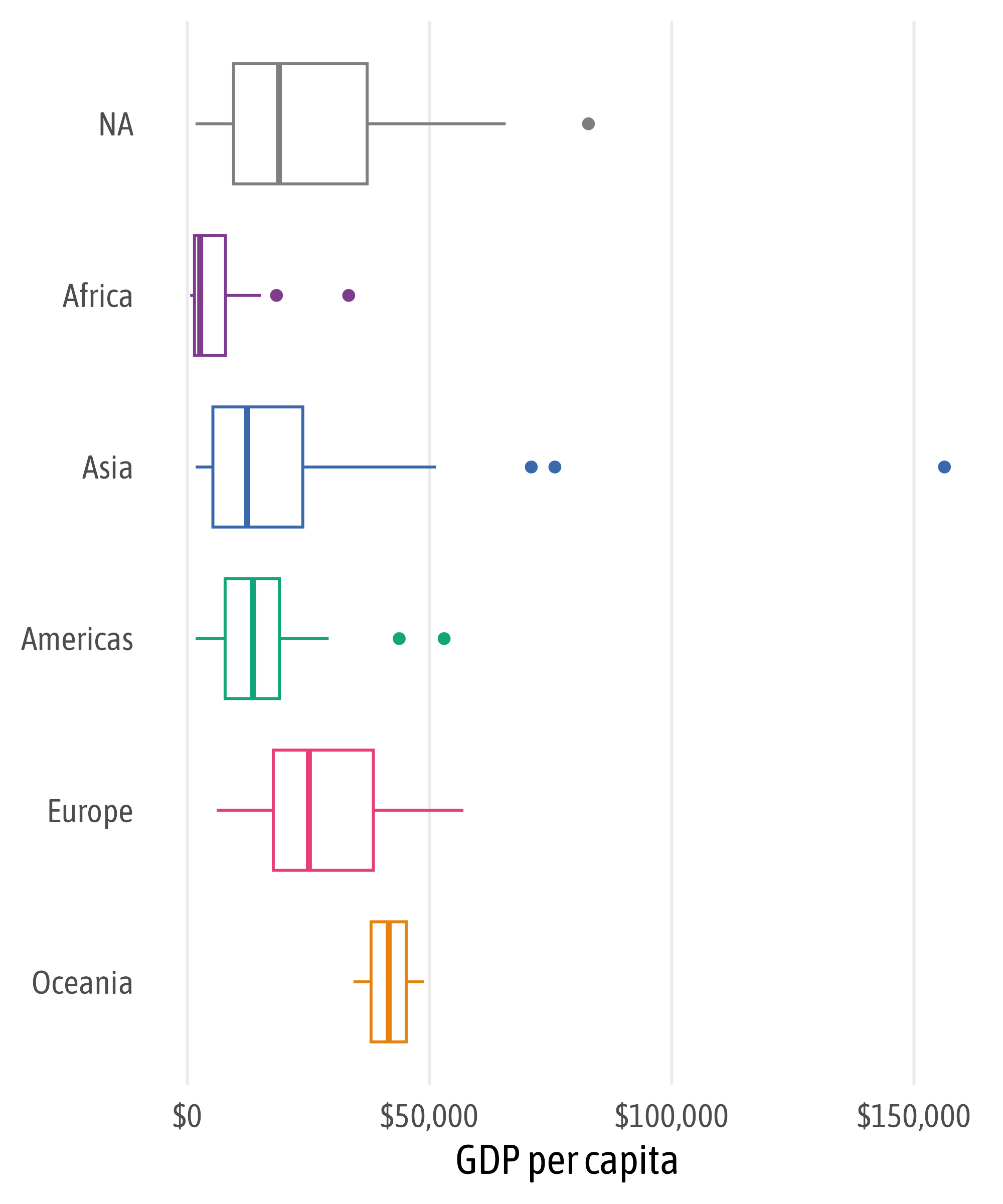
Re-use Palettes
Highlight Colors

Highlight Colors

Highlight Colors
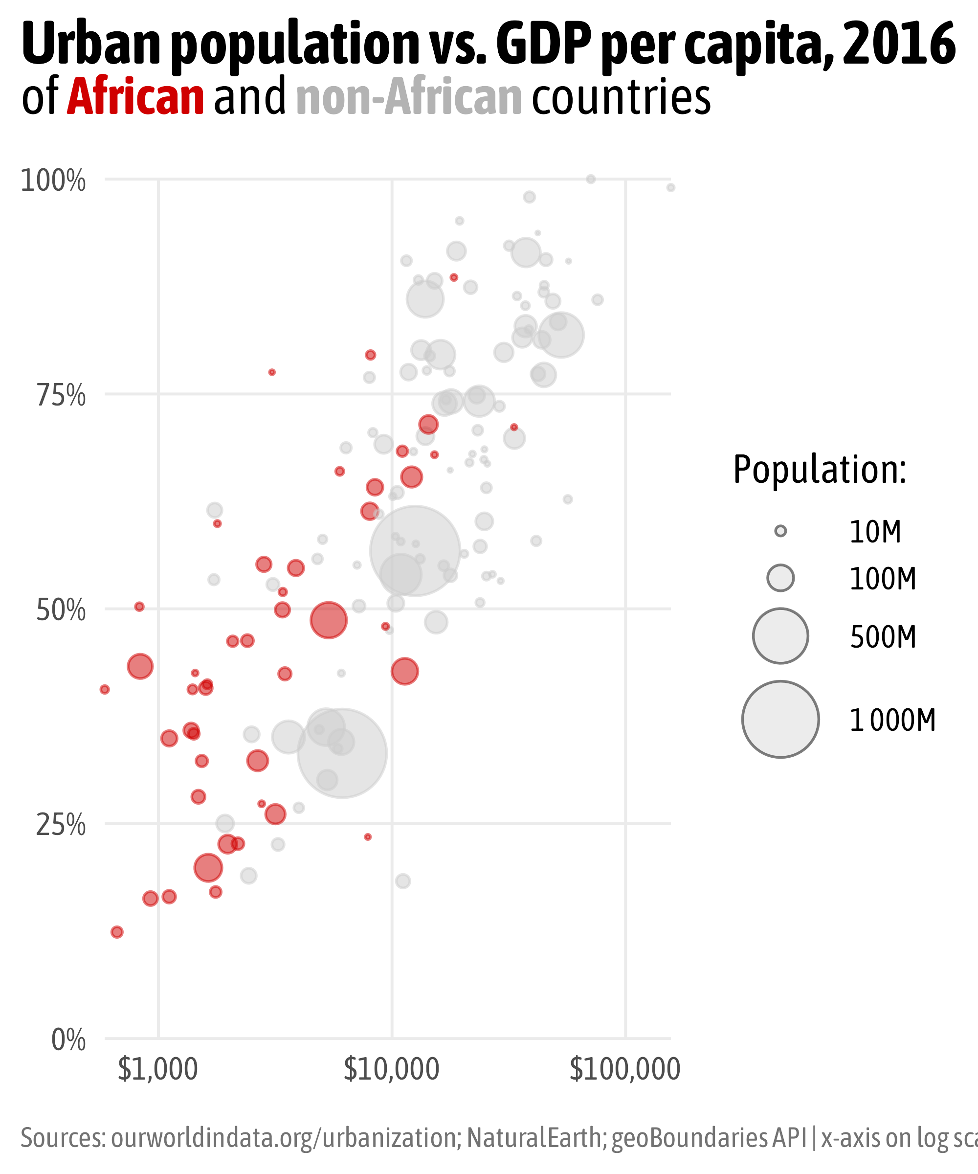
p +
  geom_point(
    aes(fill = region_un != "Africa"),
    shape = 21, alpha = .5, stroke = .7
  ) +
  scale_fill_manual(
    values = c("#D00000", "grey80")
) +
guides(fill = "none") +
labs(subtitle = "of <b style='color:#D00000;'>African</b> and <b style='color:grey70;'>non-African</b> countries") +
theme(
plot.subtitle = ggtext::element_markdown(
margin = margin(t = -15, b = 20),
size = rel(1.3)
)
)
Highlight Colors
p +
  geom_point(
    aes(fill = region_un != "Africa",
        color = after_scale(fill)),
    shape = 21, alpha = .5, stroke = .7
  ) +
  scale_fill_manual(
    values = c("#D00000", "grey80")
  ) +
  labs(subtitle = "of <b style='color:#D00000;'>African</b> and <b style='color:grey70;'>non-African</b> countries") +
  guides(fill = "none") +
  theme(
    plot.subtitle = ggtext::element_markdown(
      margin = margin(t = -15, b = 20),
      size = rel(1.3)
    )
  )
Highlight Colors
pal_hl <- c("#7754BF", "#28A74D", "grey80")

p +
  geom_point(
    data = df_world,
    aes(fill = cont_lumped,
        color = after_scale(clr_darken(fill, .3))),
    shape = 21, alpha = .5, stroke = .7
  ) +
  scale_fill_manual(values = pal_hl) +
  labs(subtitle = "of <b style='color:#7754BF;'>Asian</b> and <b style='color:#28A74D;'>European</b> countries compared to all <span style='color:grey60;'>other countries</span>") +
  guides(fill = "none") +
  theme(
    plot.subtitle = ggtext::element_markdown(
      margin = margin(t = -15, b = 20),
      size = rel(1.3)
    )
  )
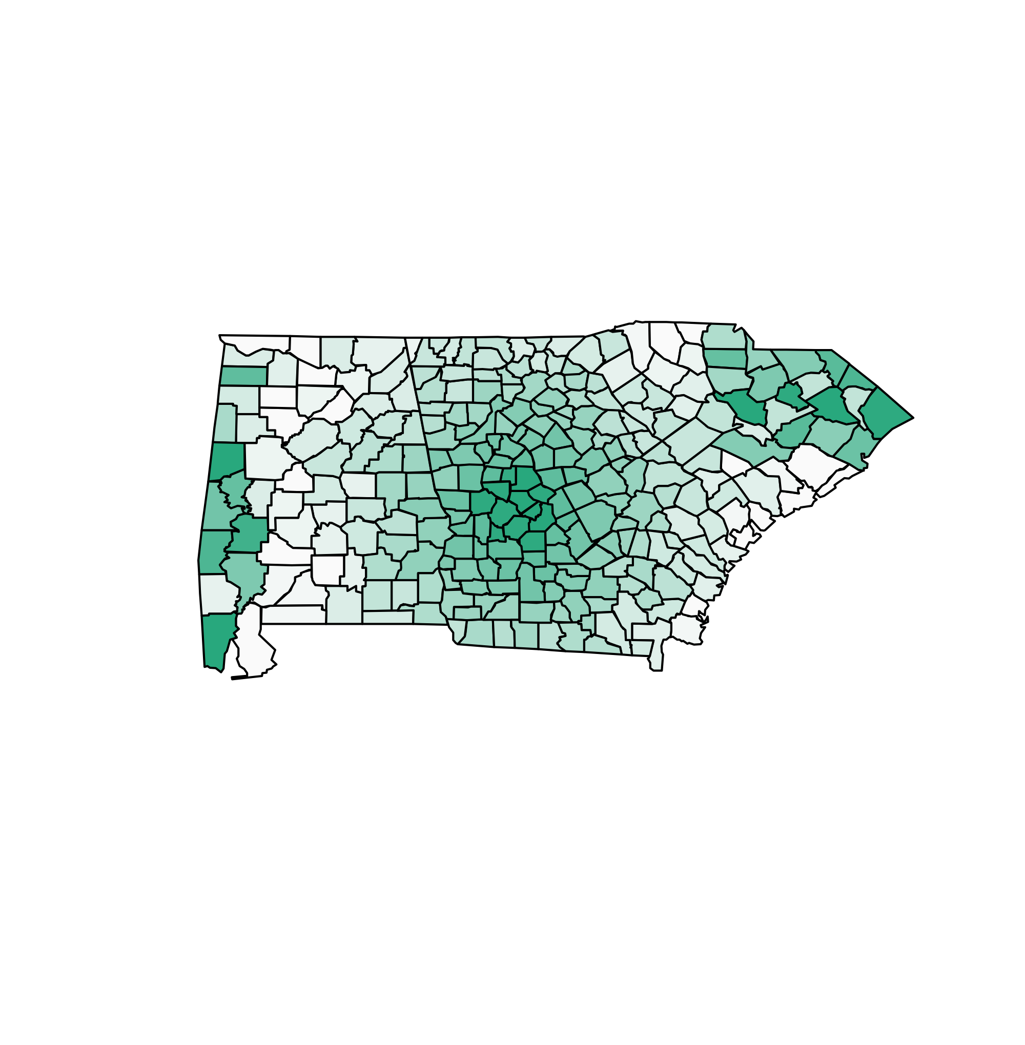
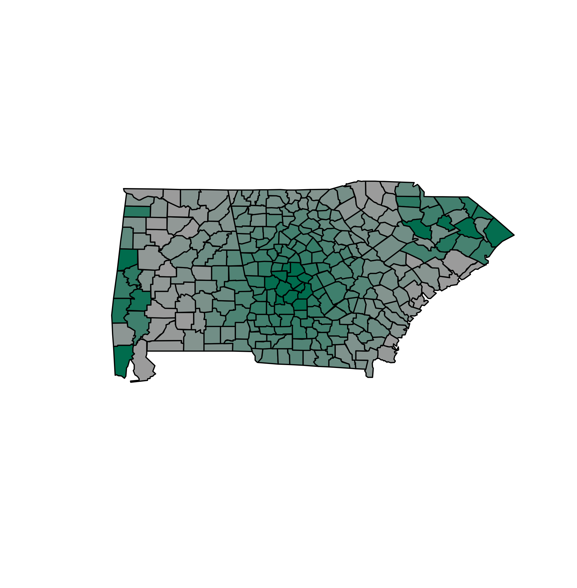
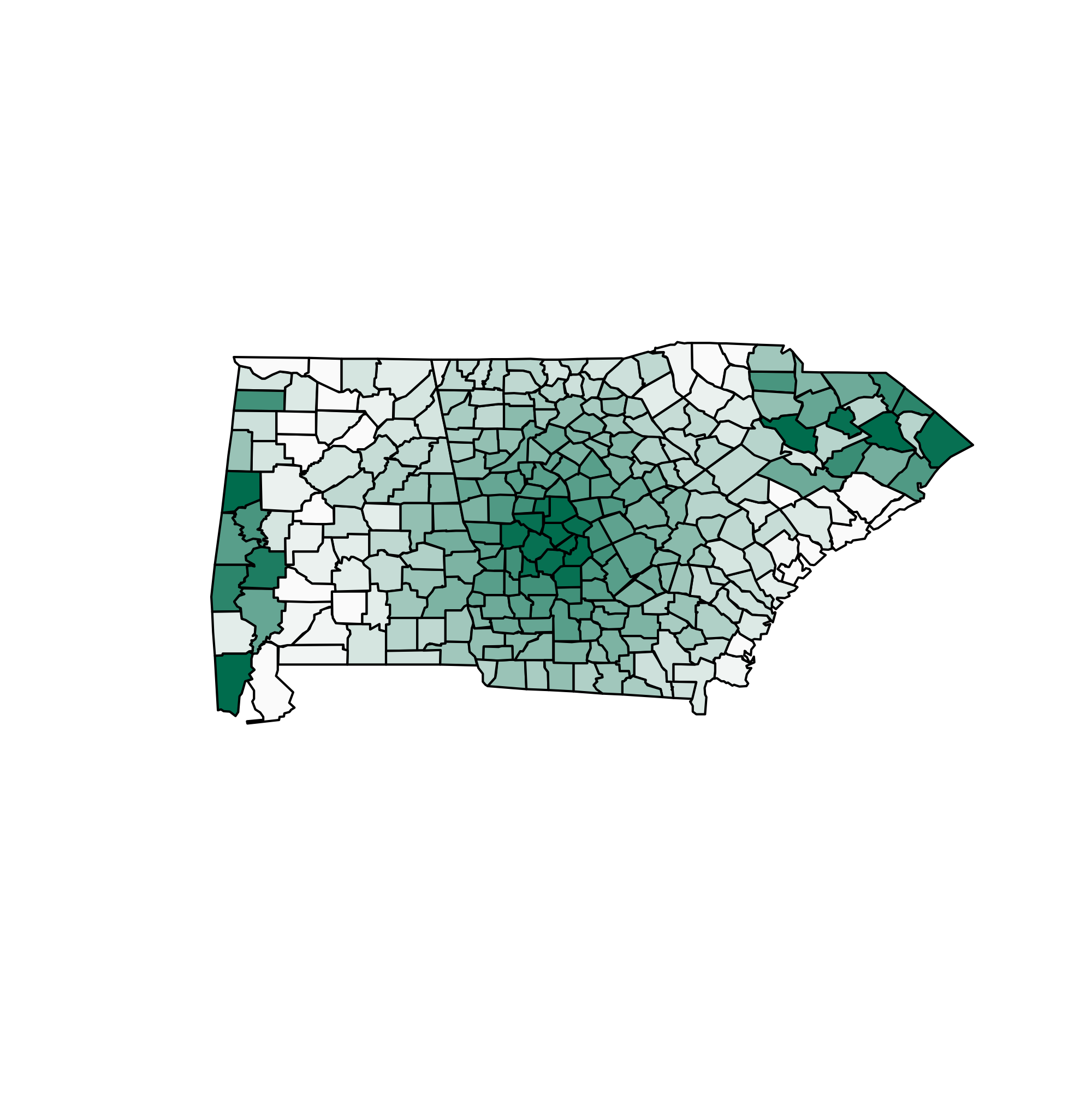
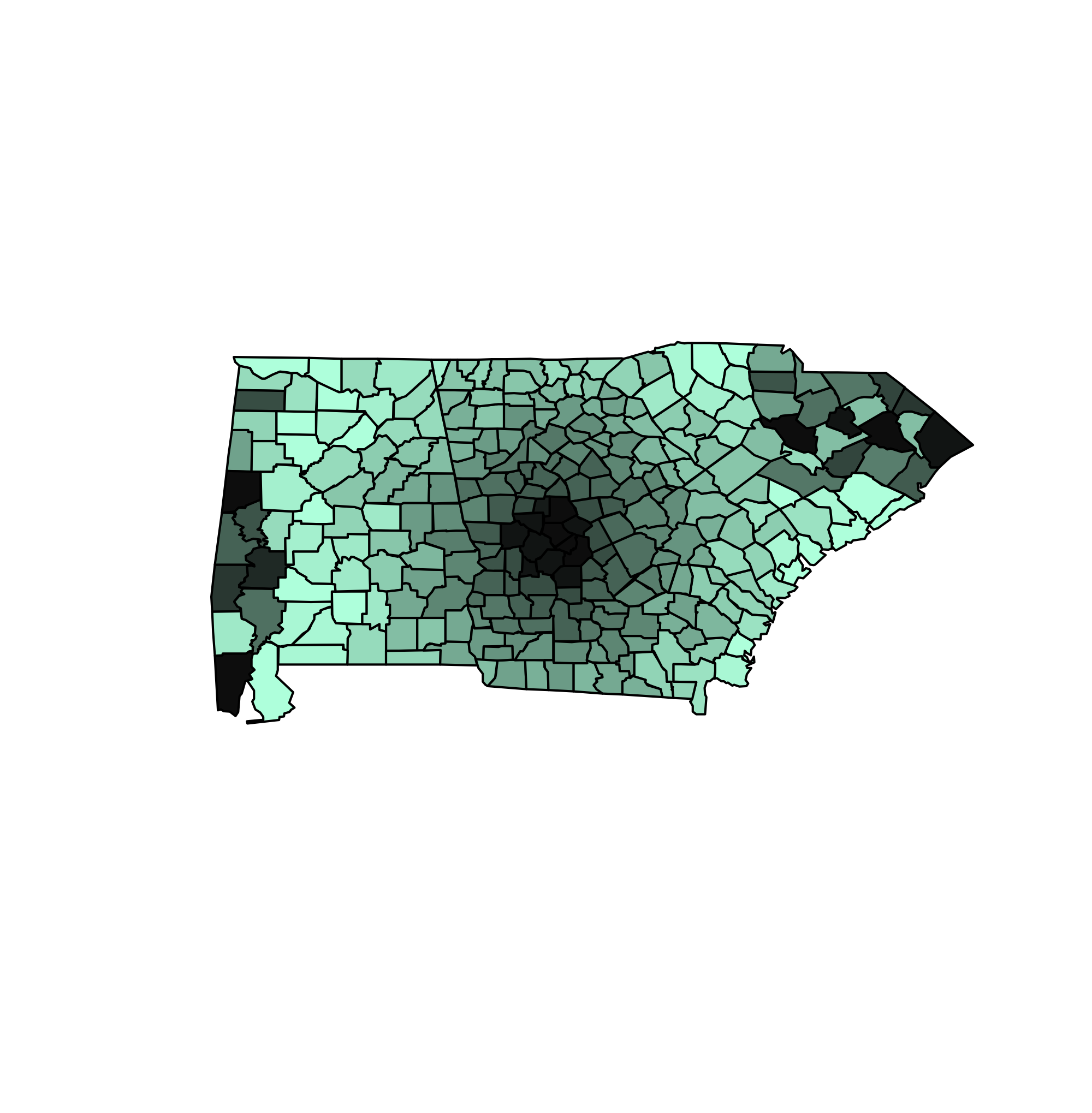
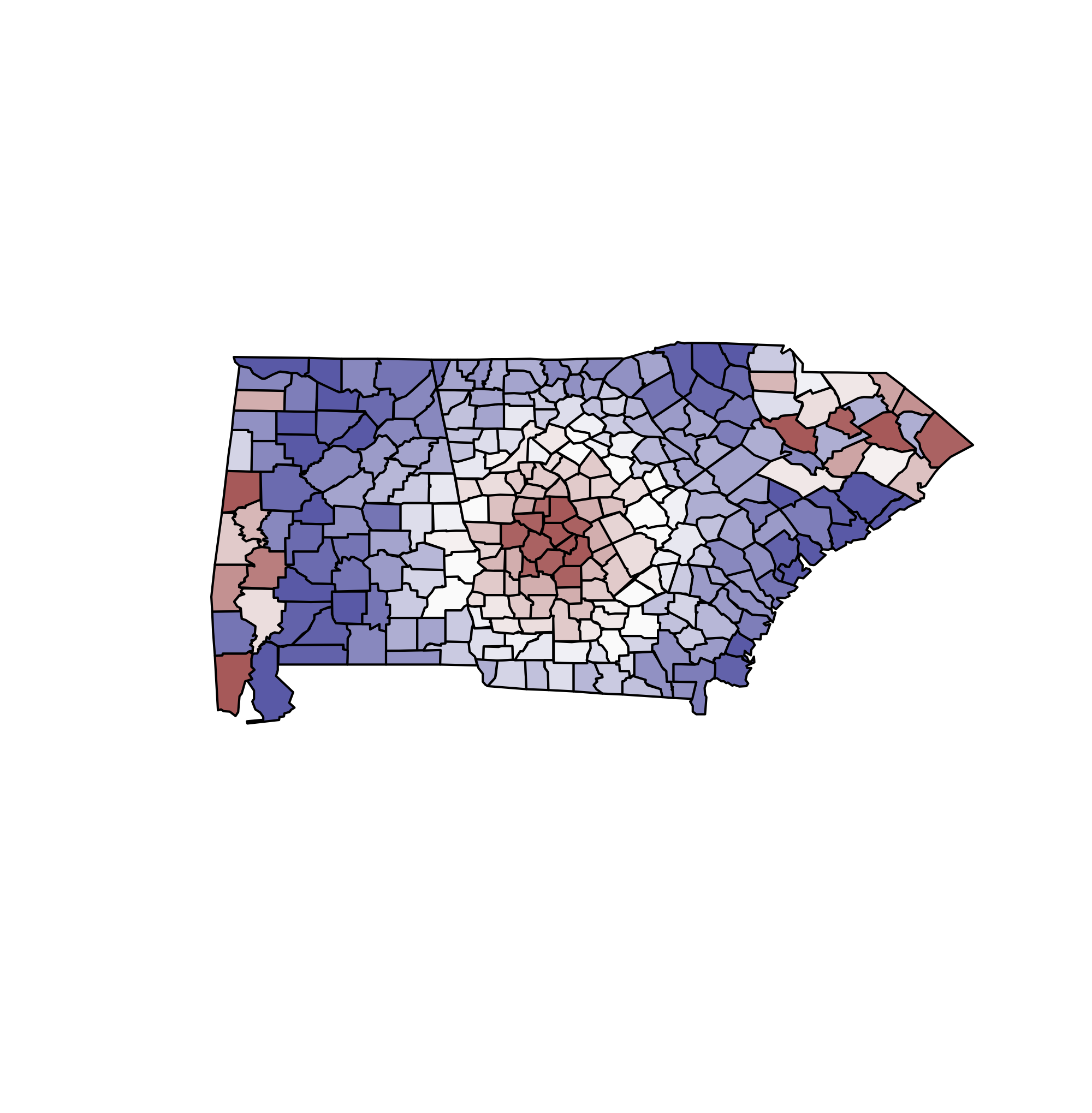
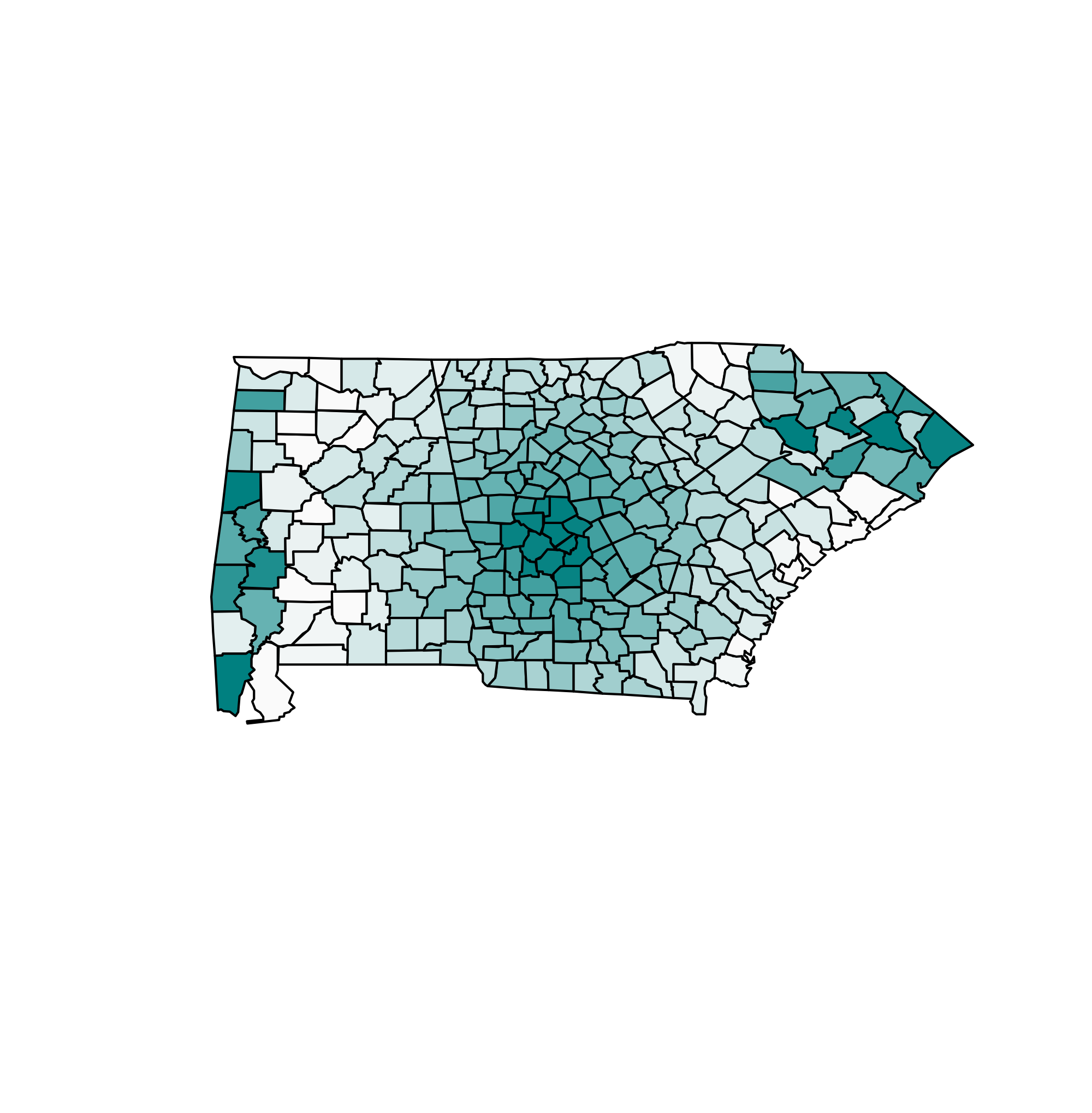
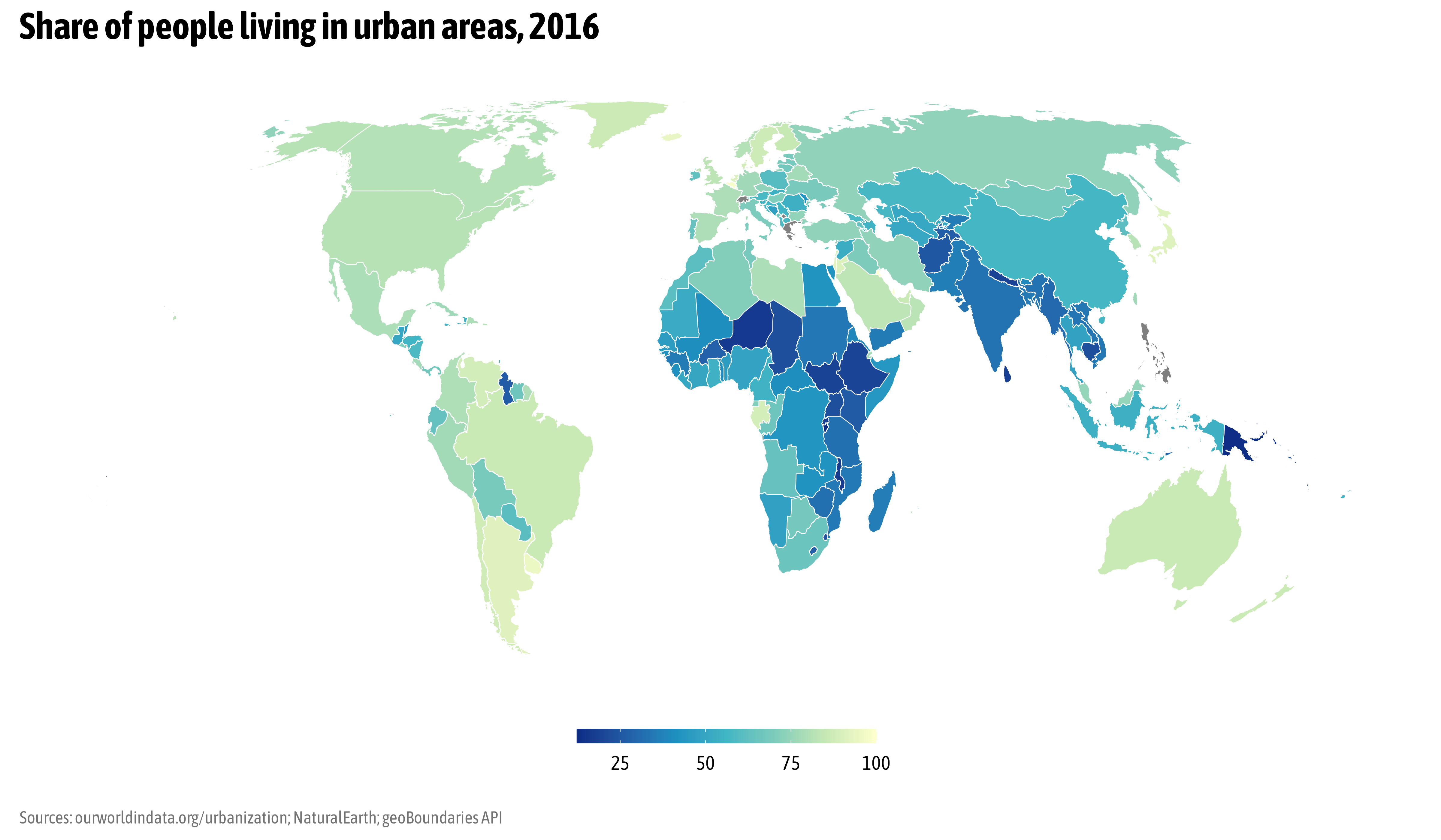
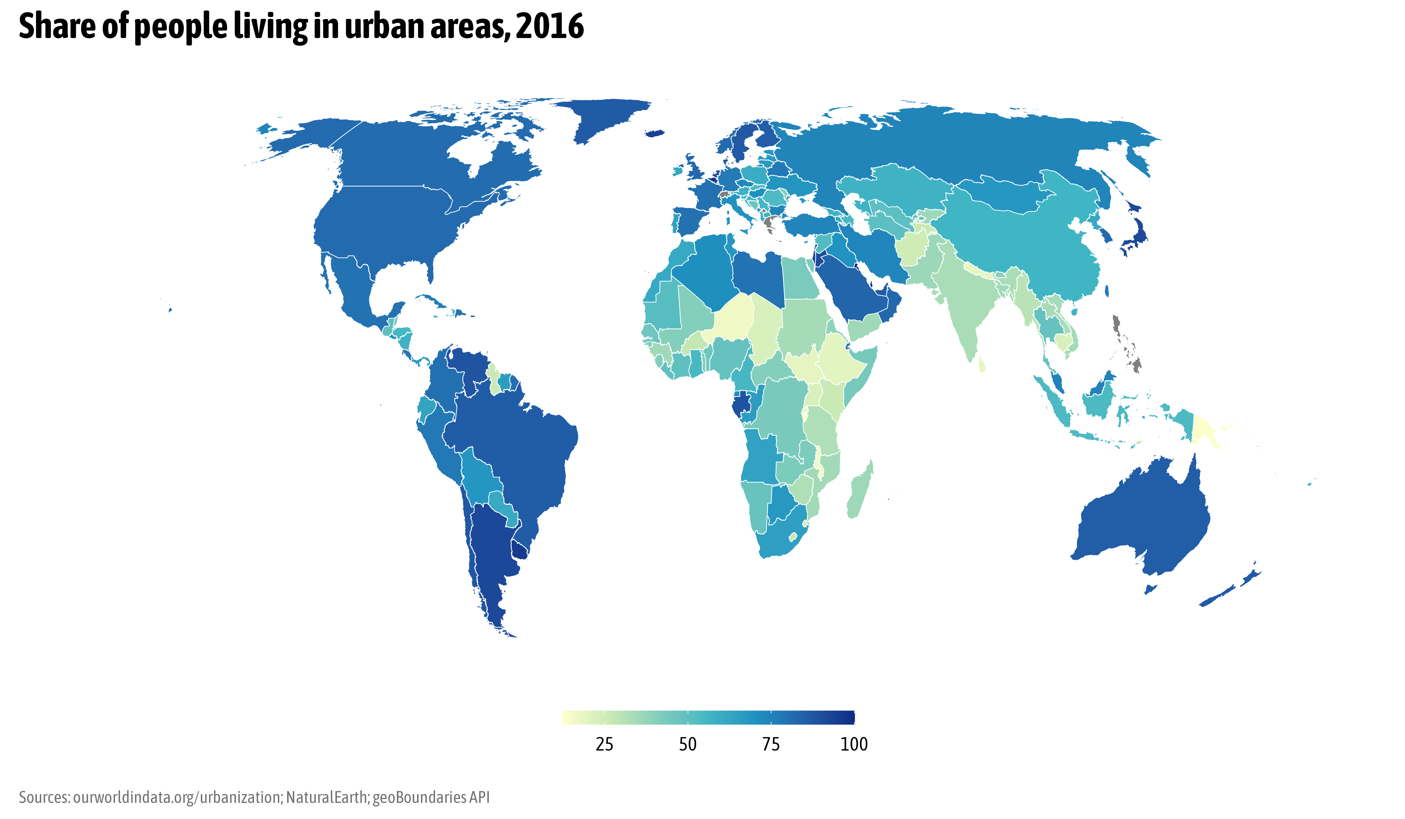
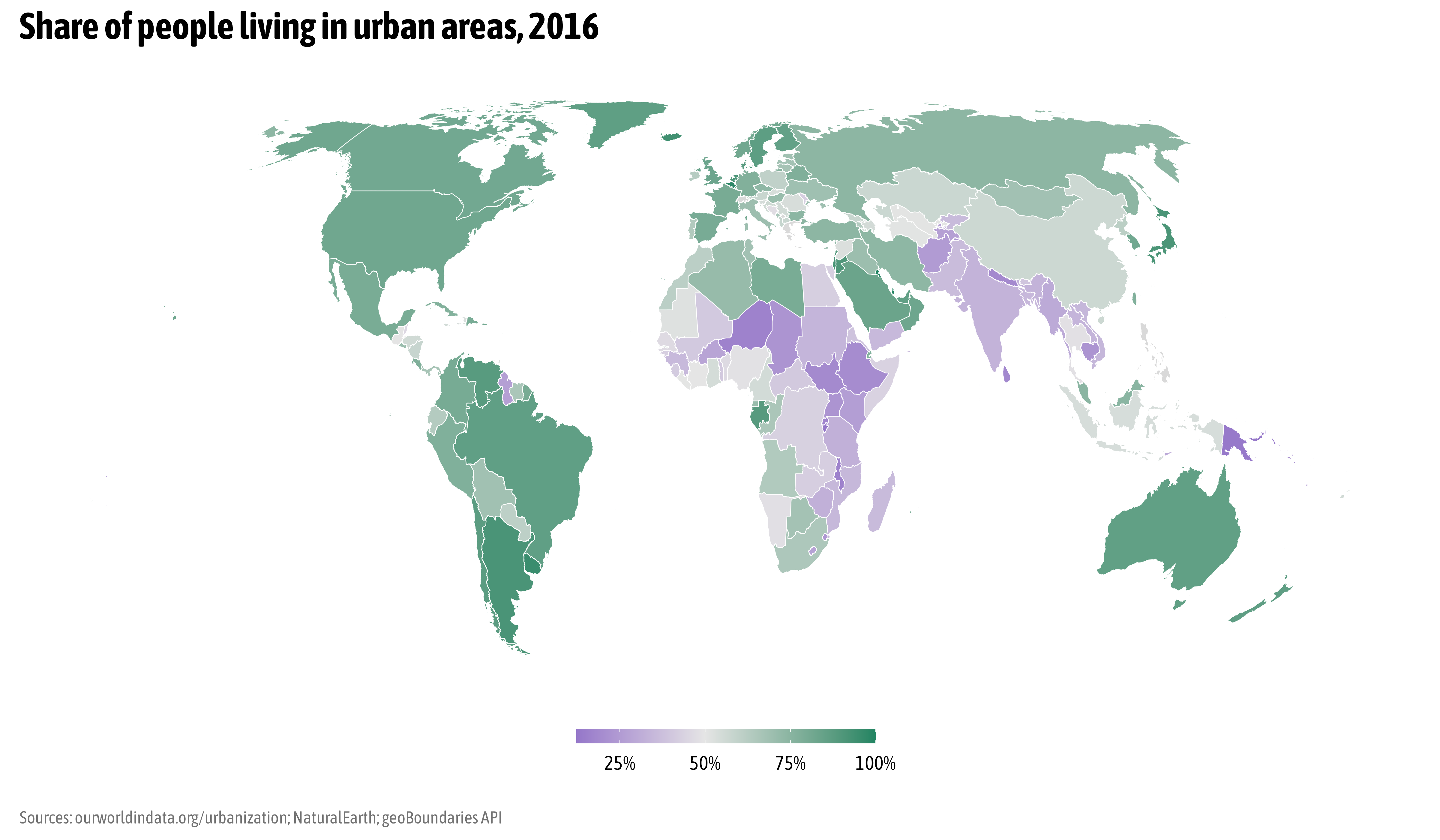
The Map
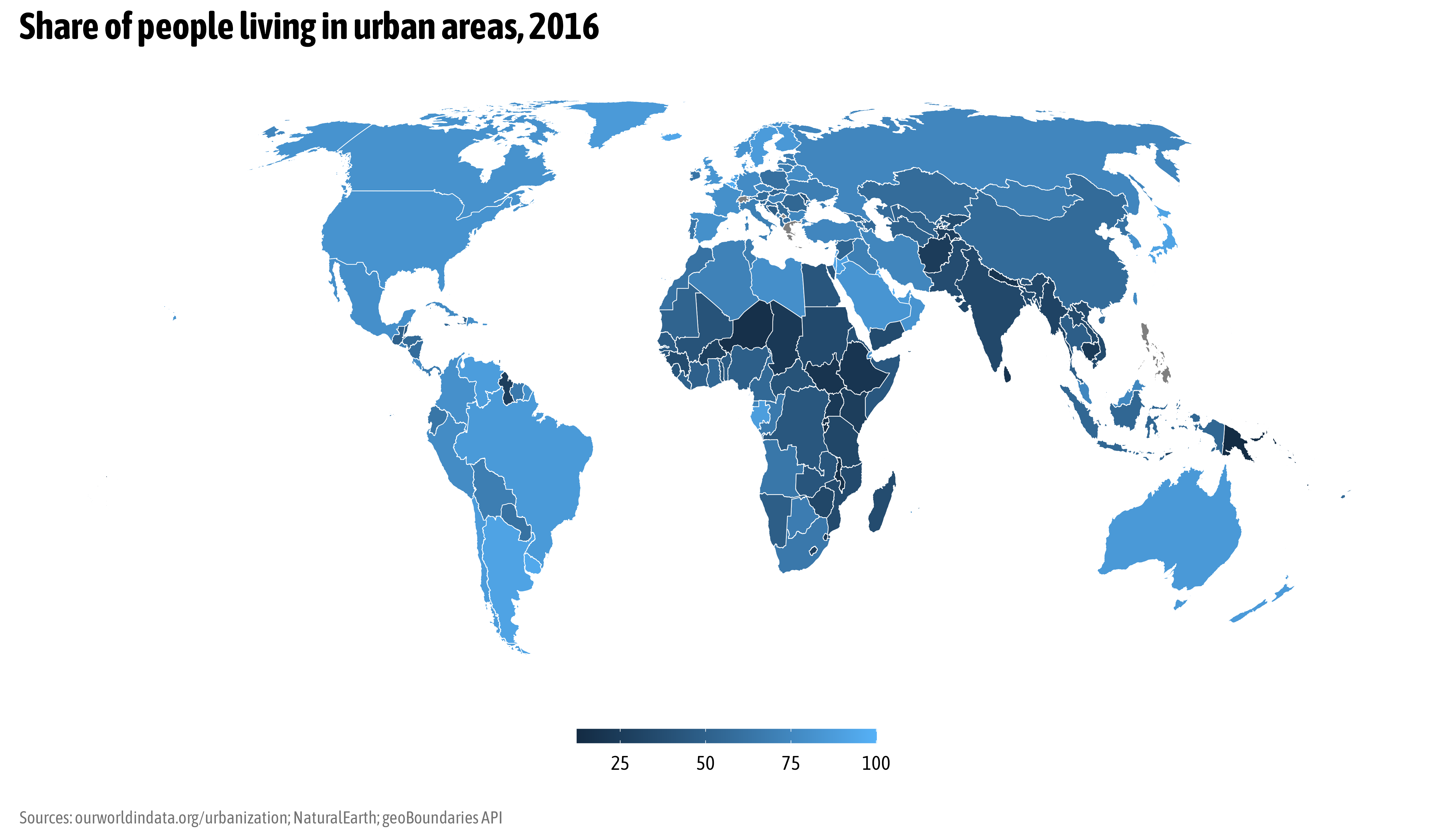
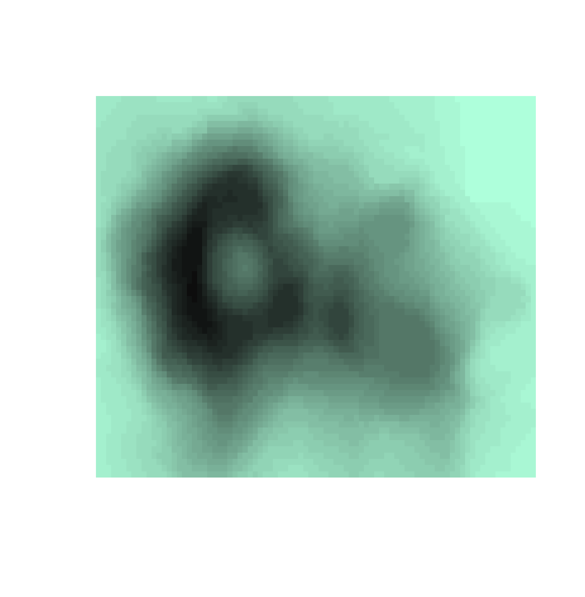
A Sequential Palette
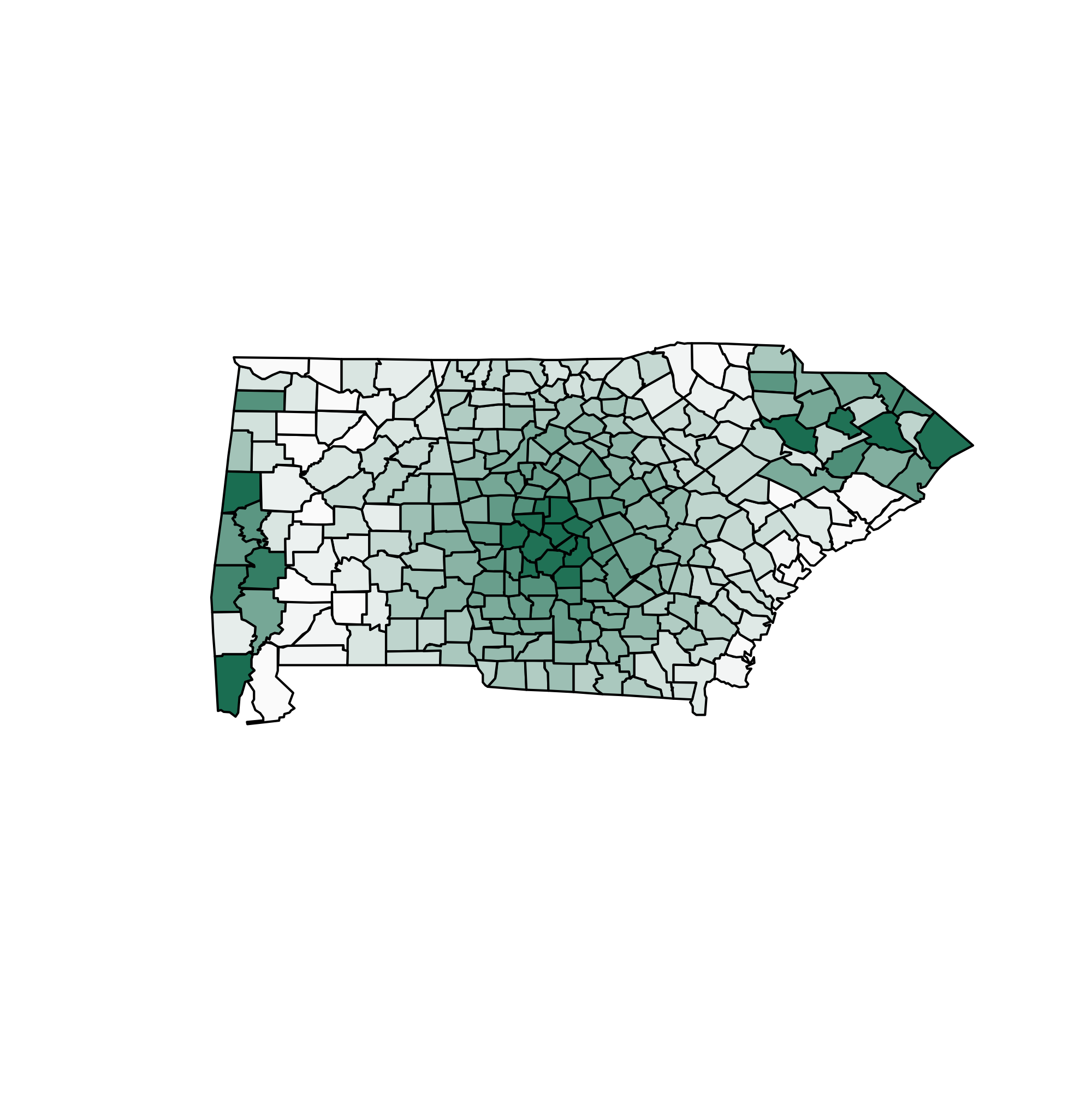
A (Reversed) Sequential Palette
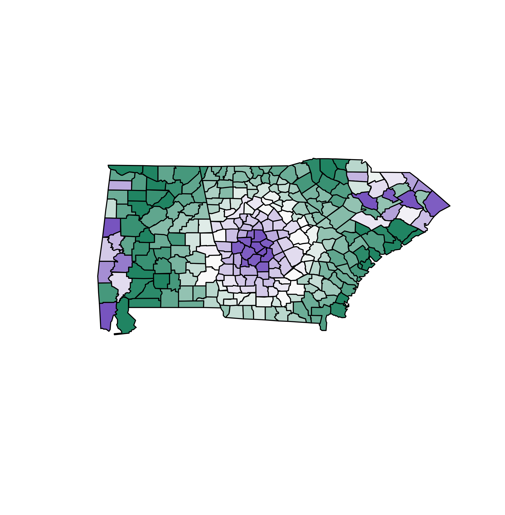
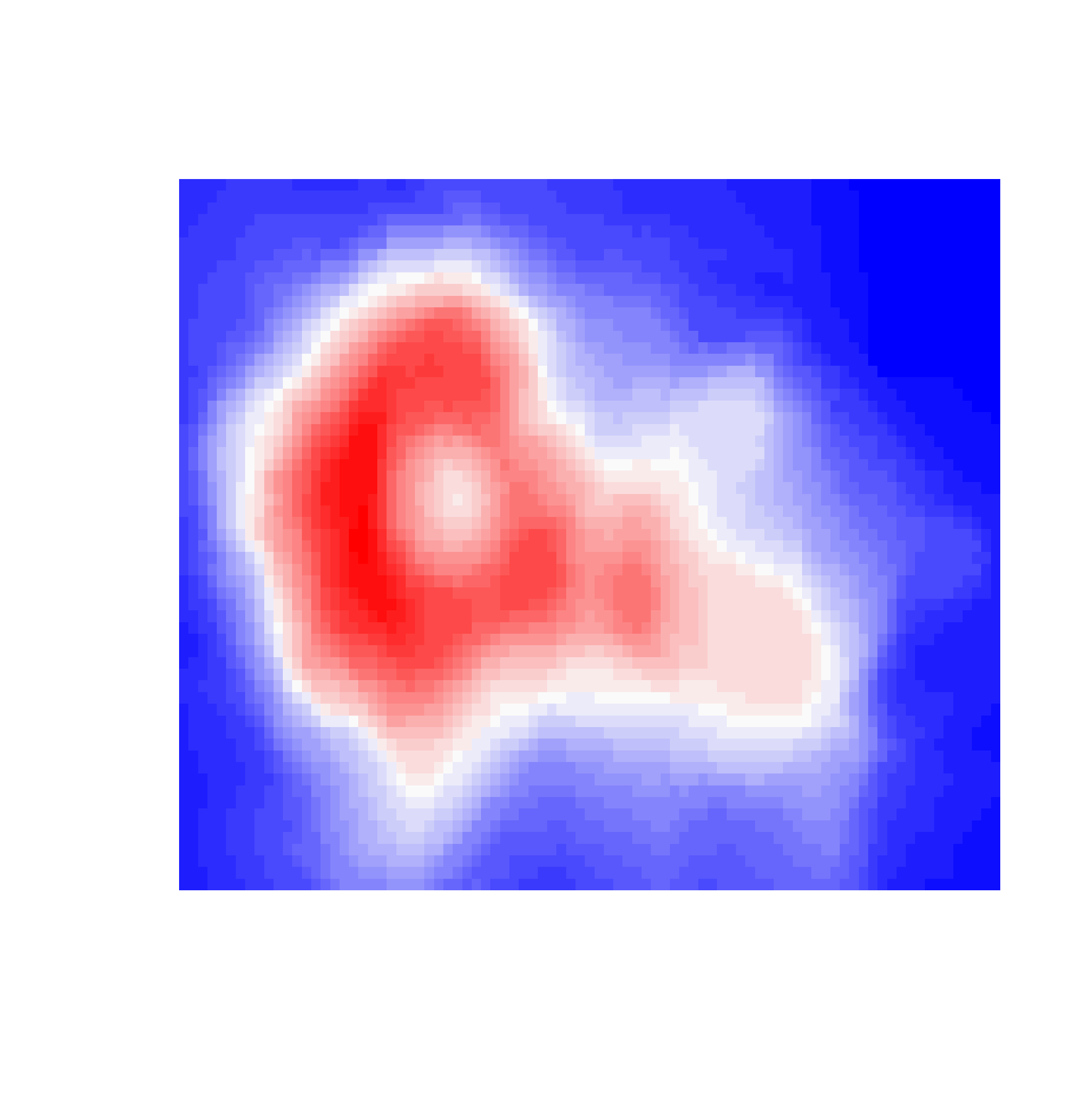
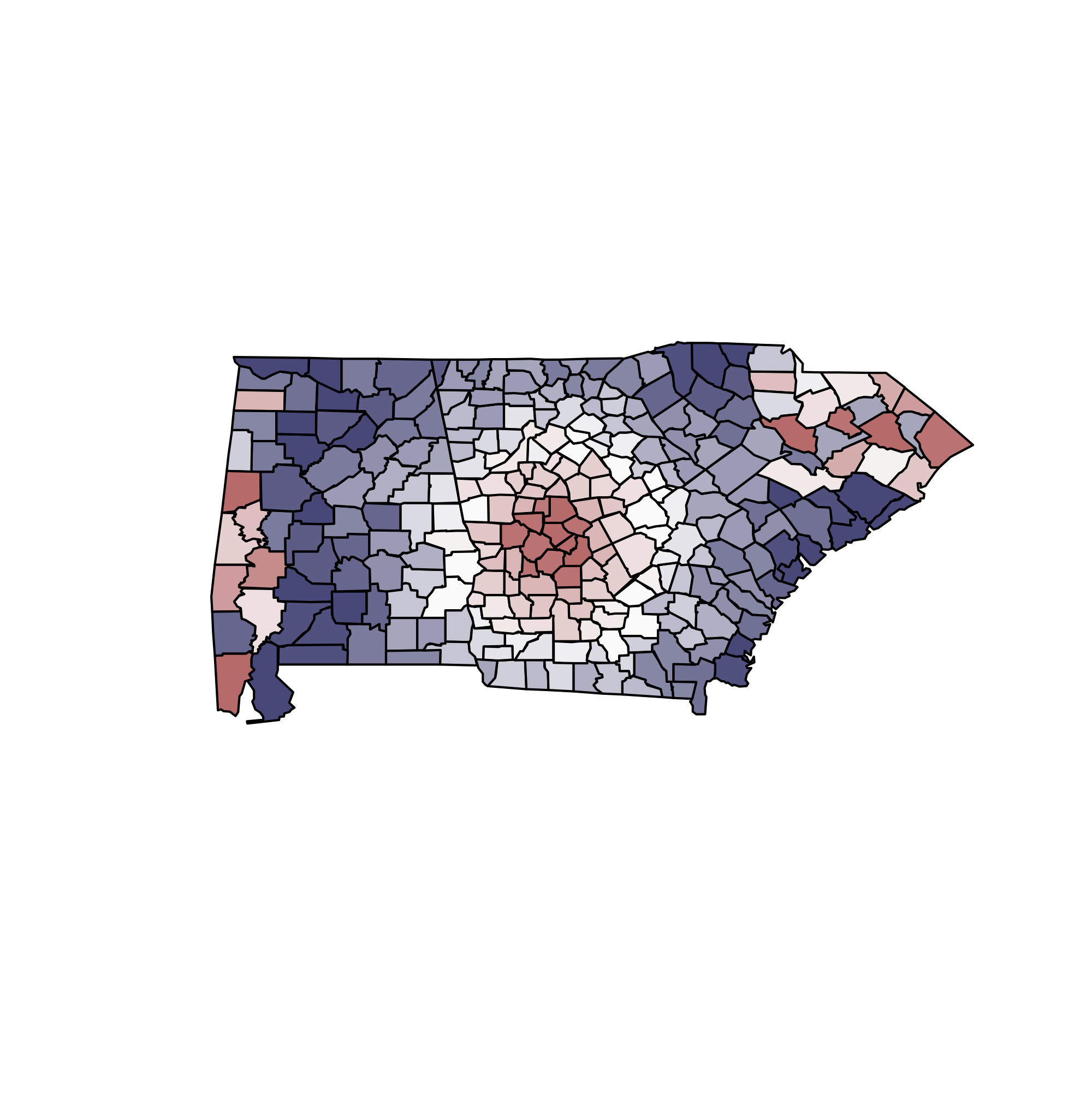
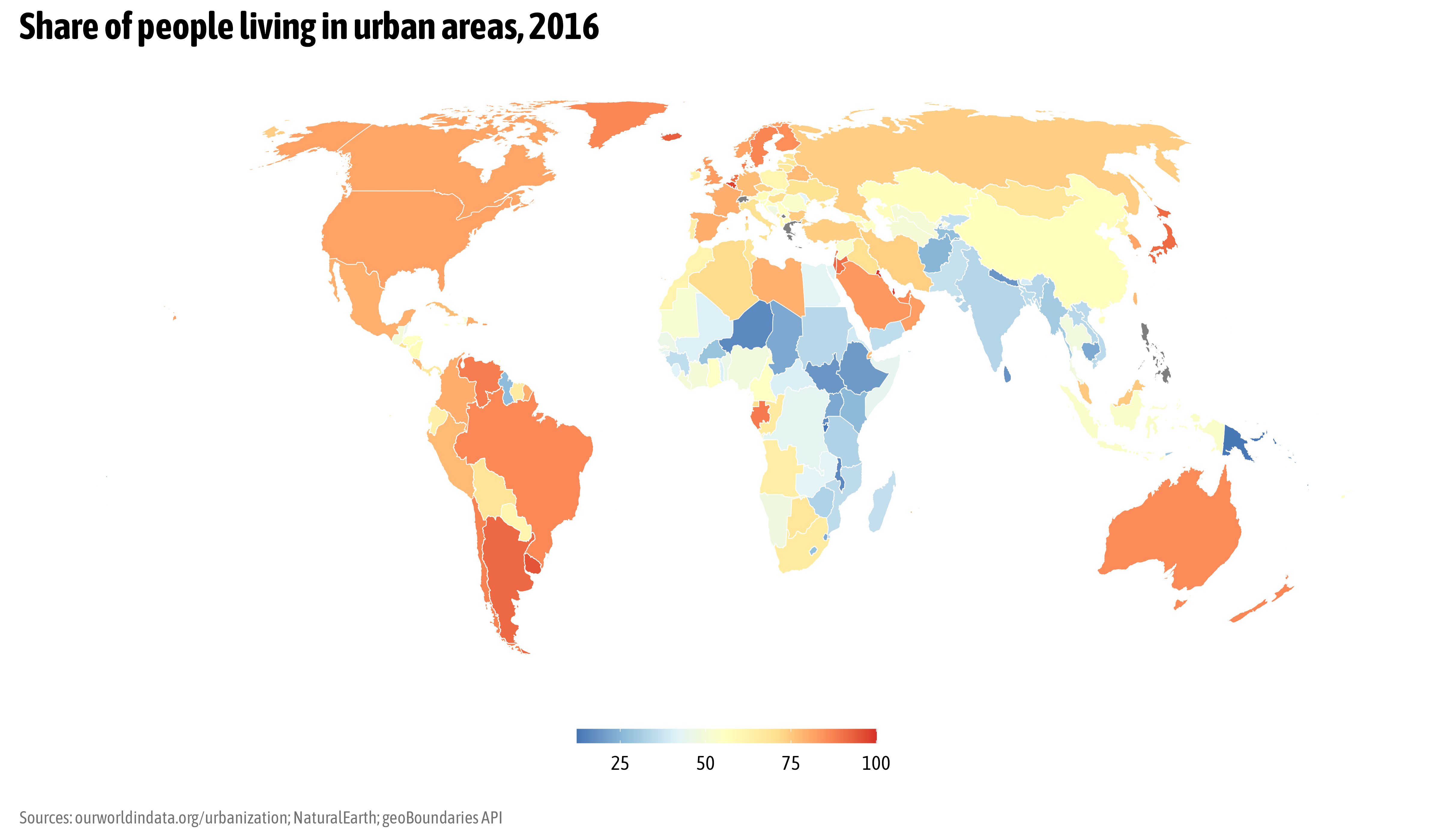
A Diverging Palette
A (Reversed) Diverging Palette
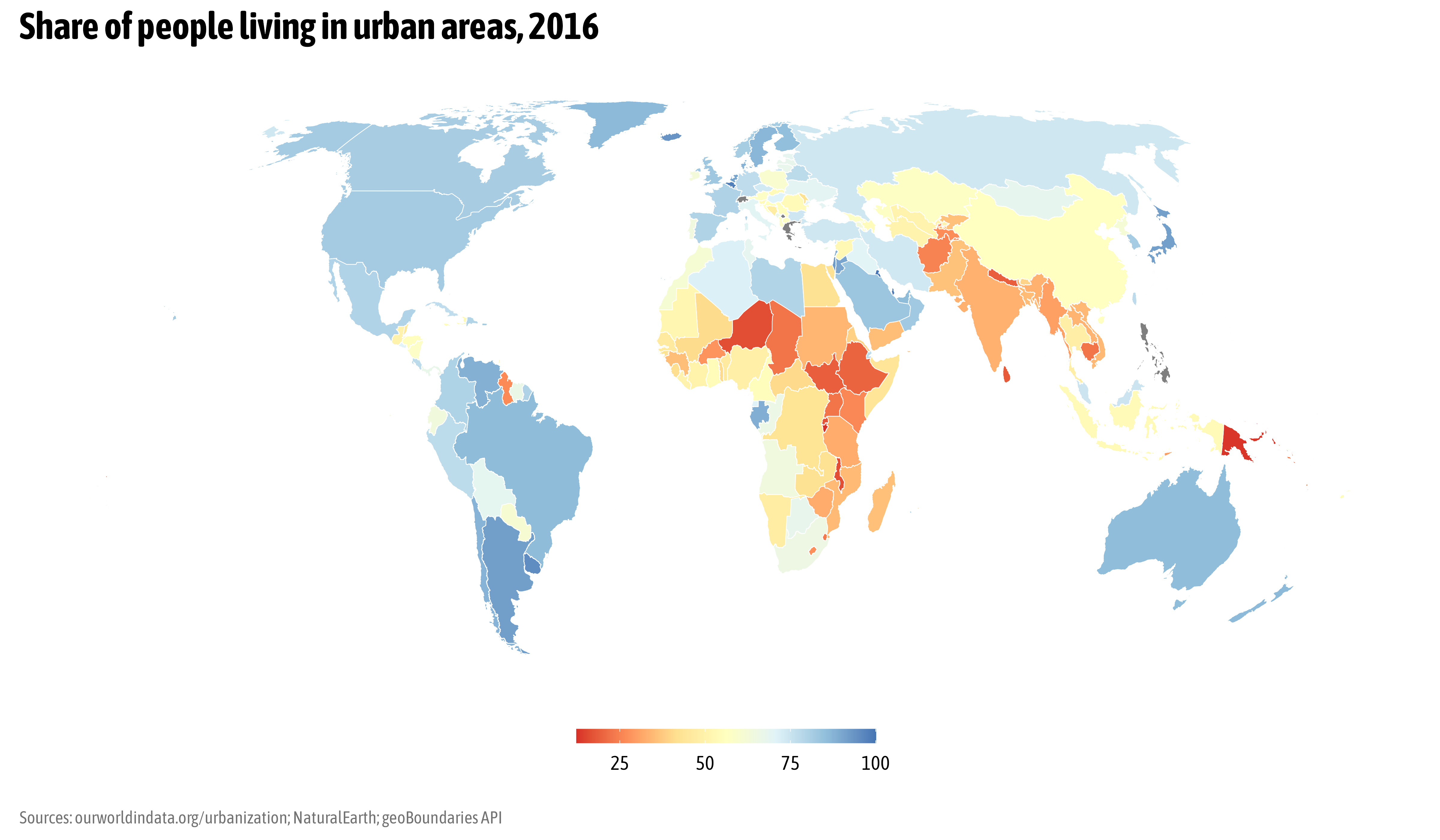
A (Fixed) Diverging Palette

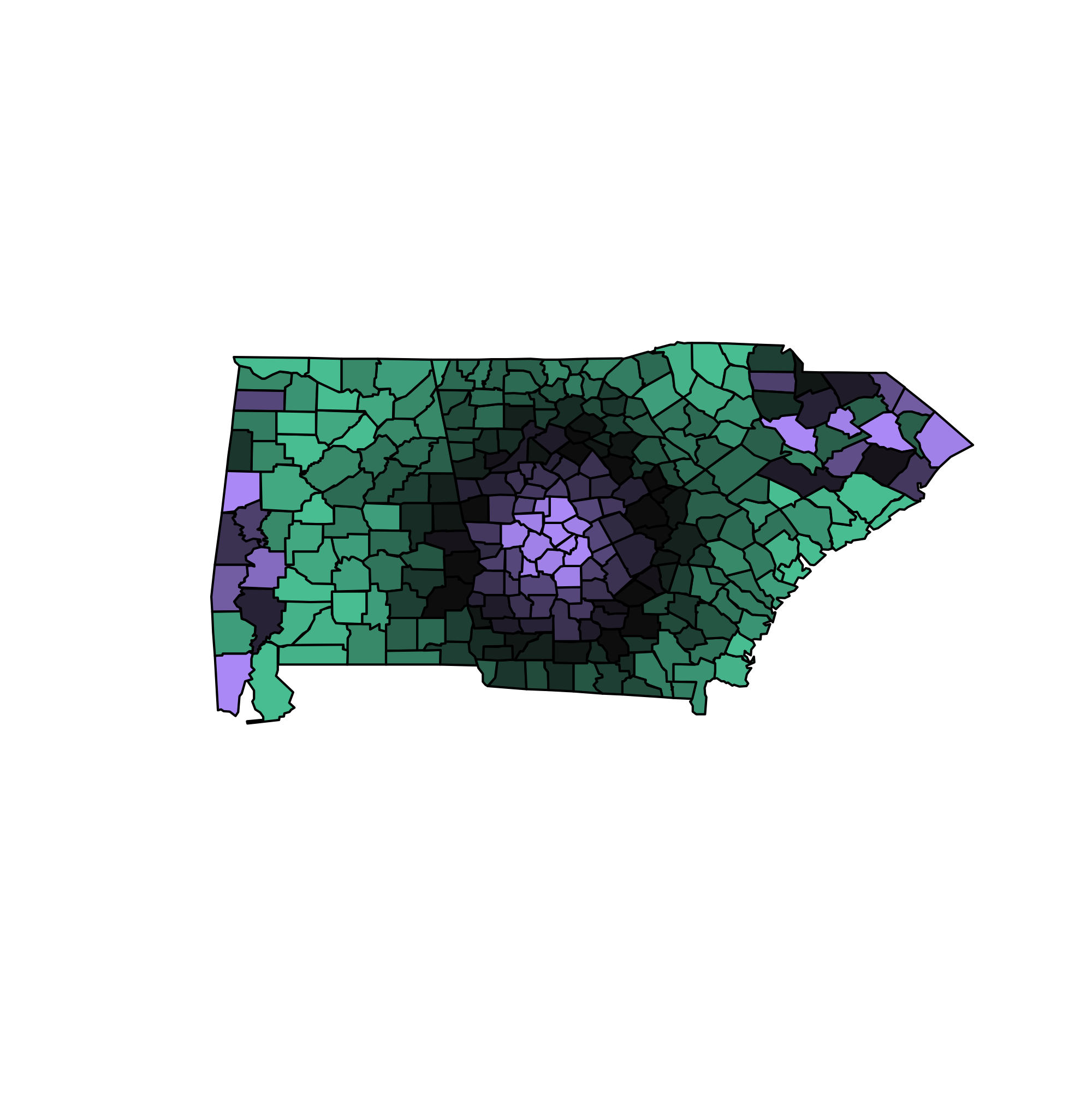
A (Styled) Diverging Palette
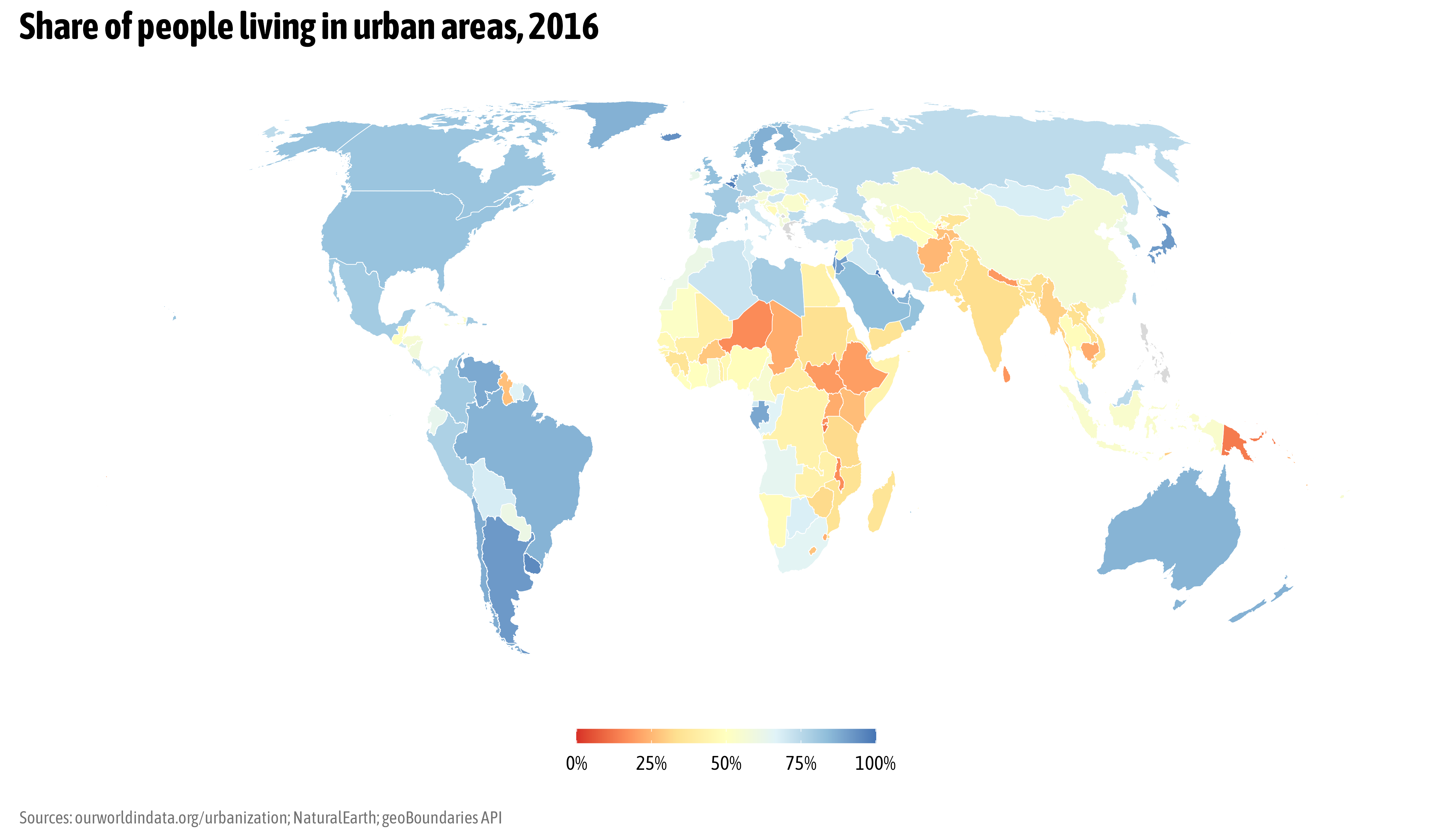
A (Custom) Diverging Palette
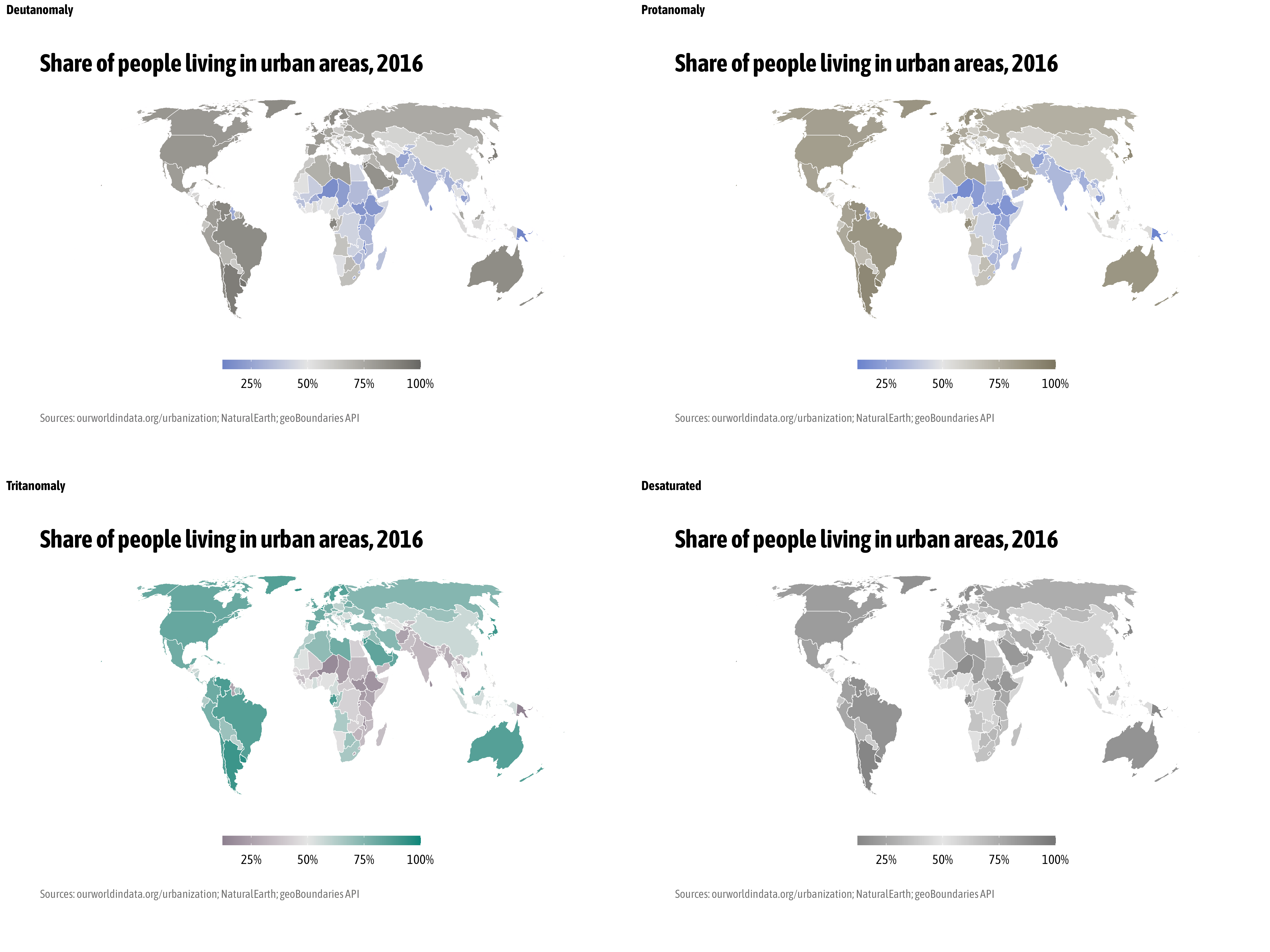
Test Color Palettes
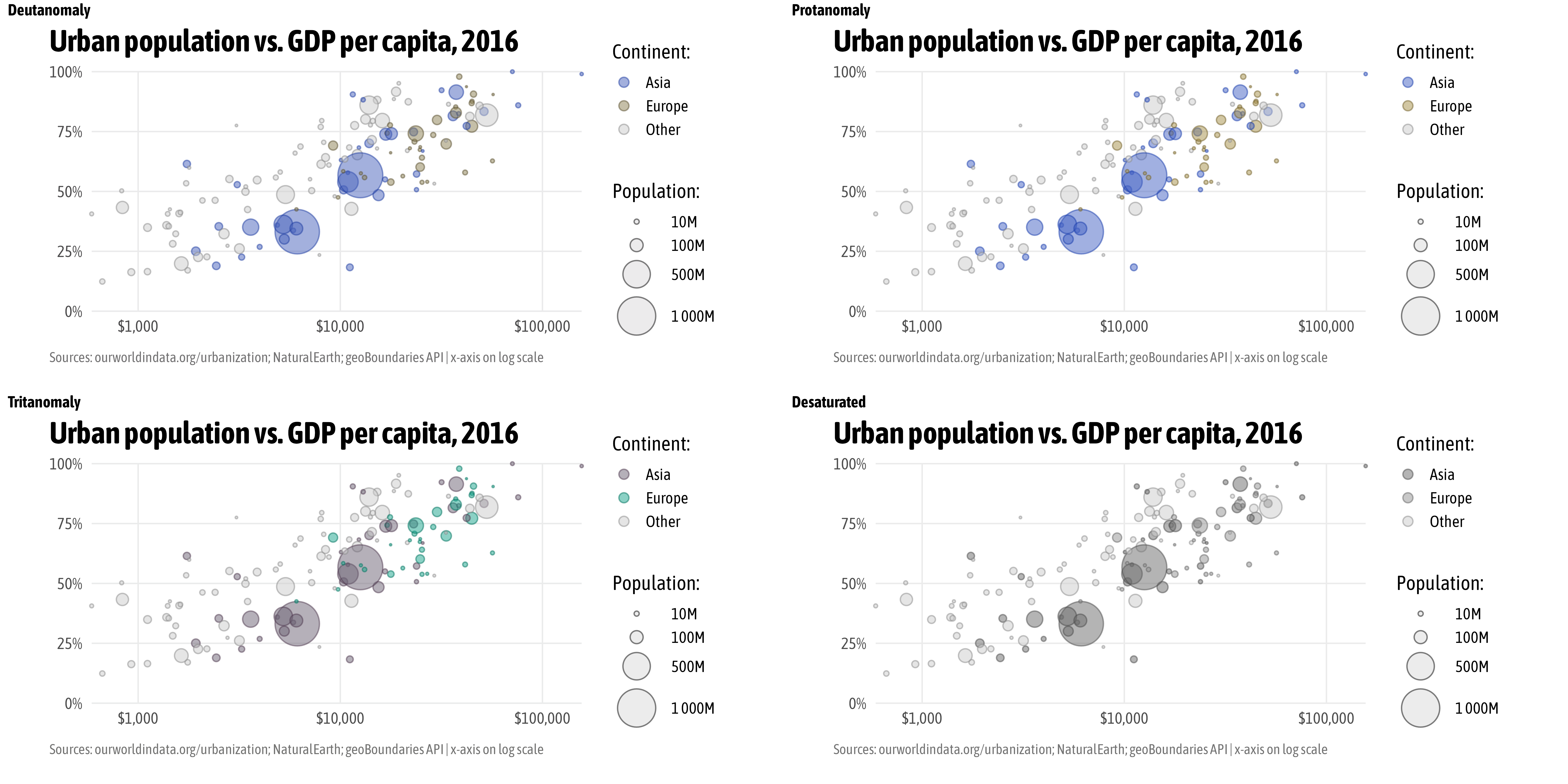
Test Color Palettes
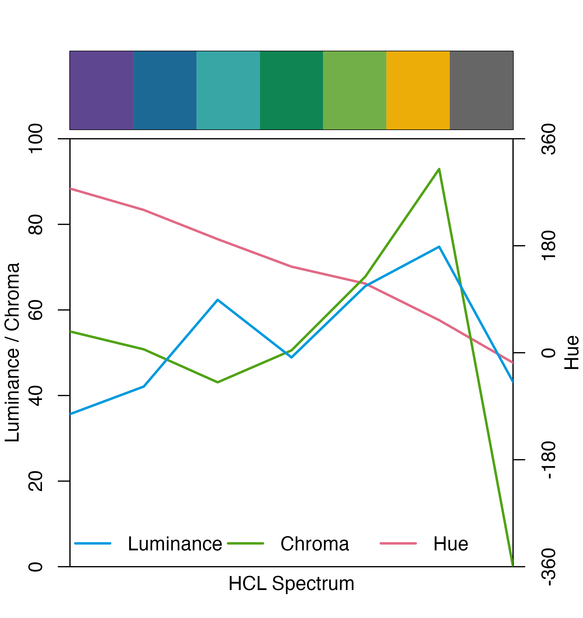
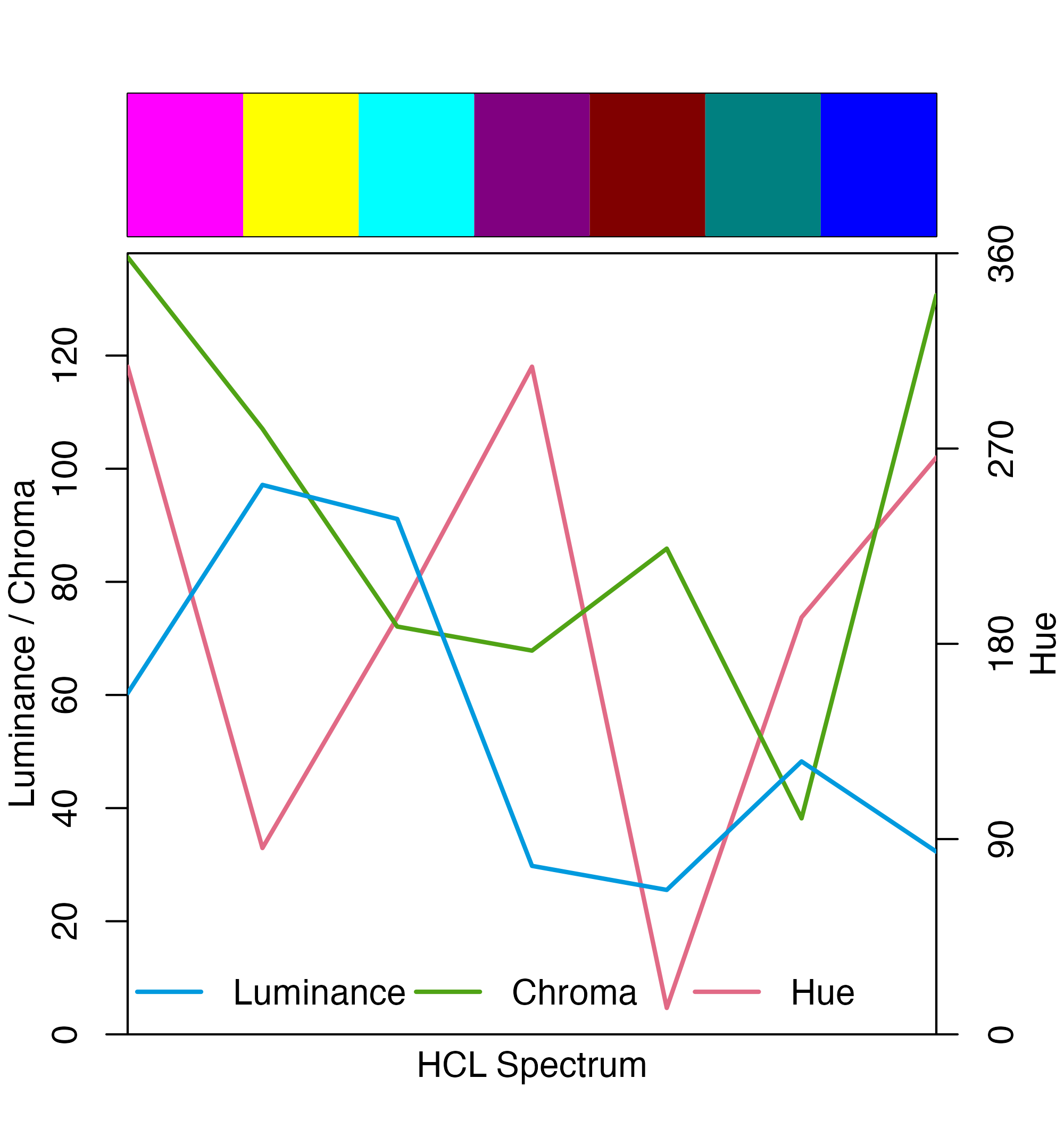
Evaluate HCL Space
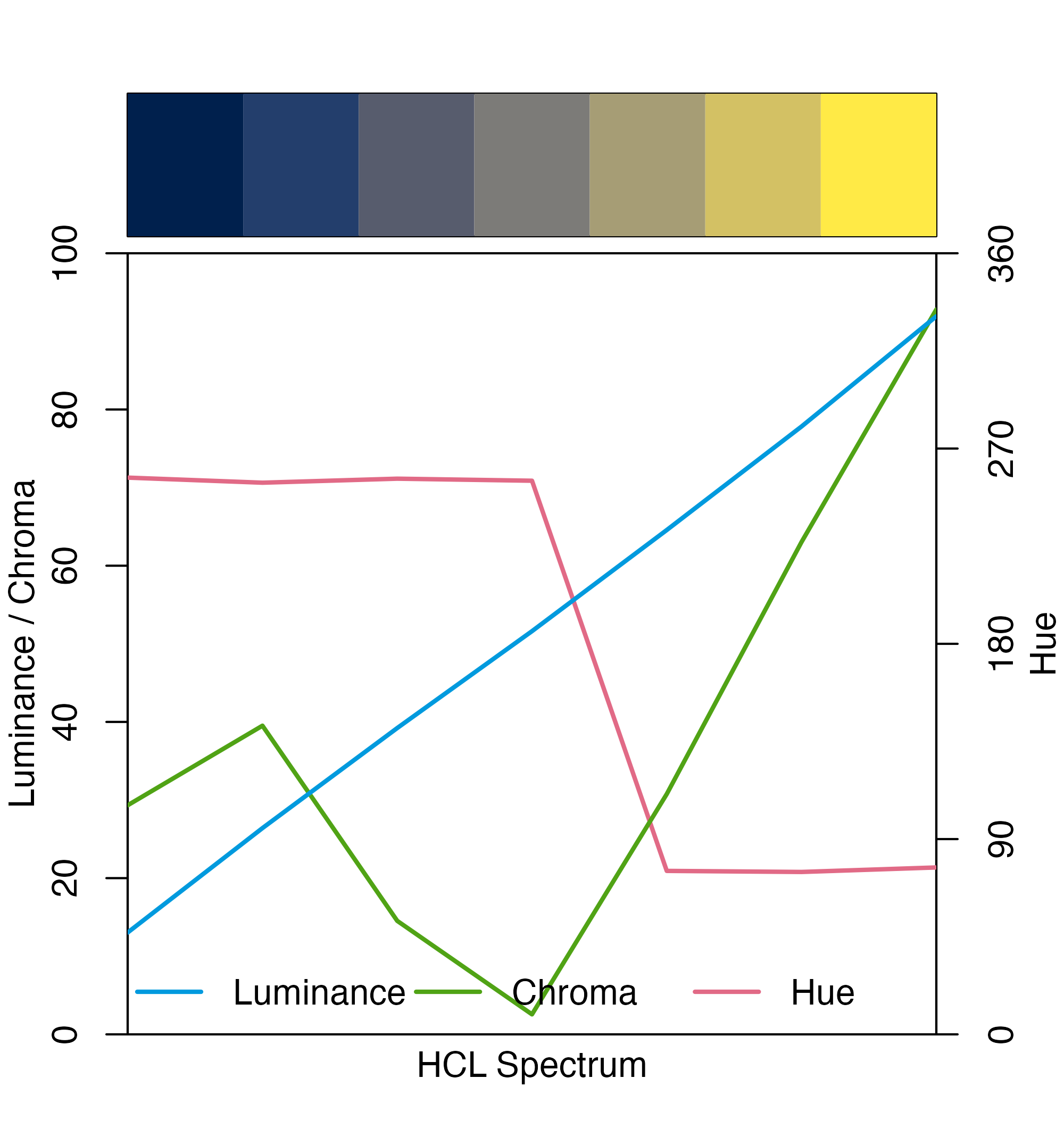
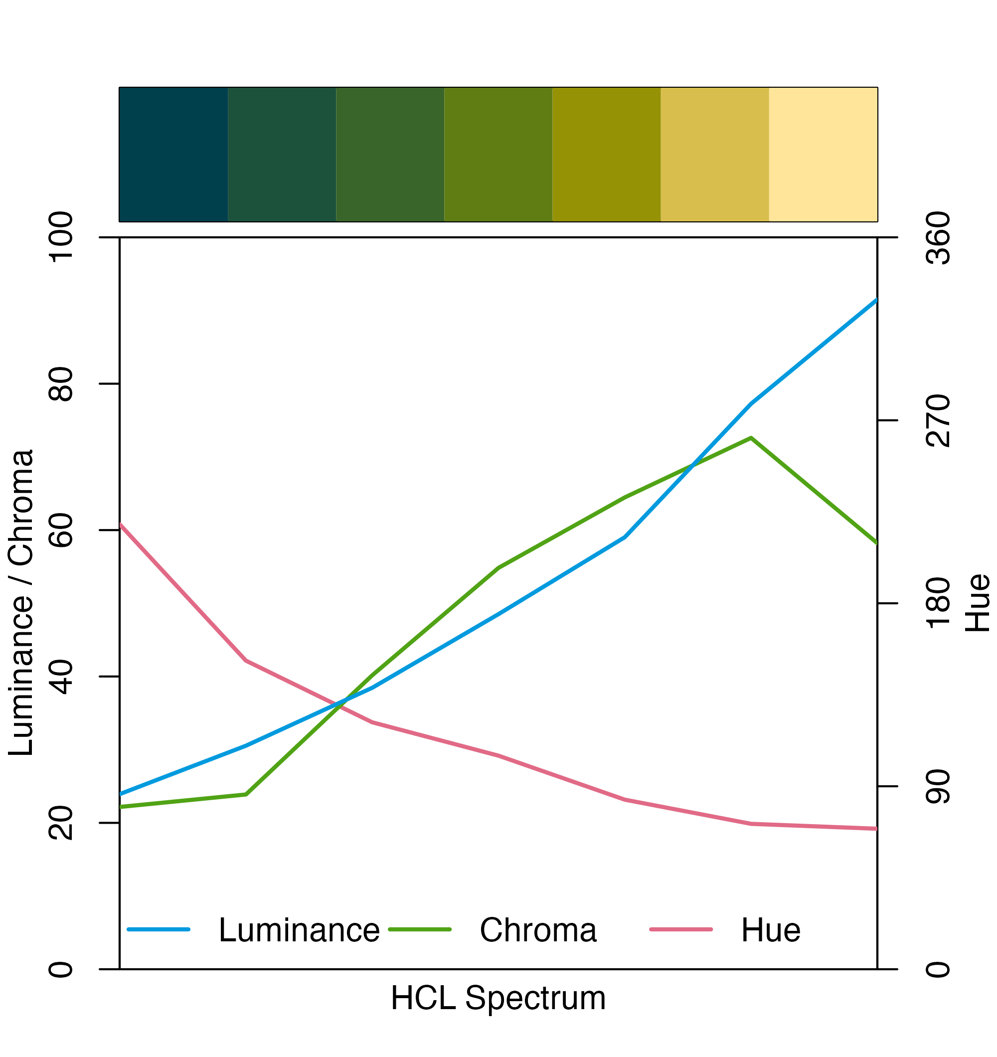
Evaluate HCL Space
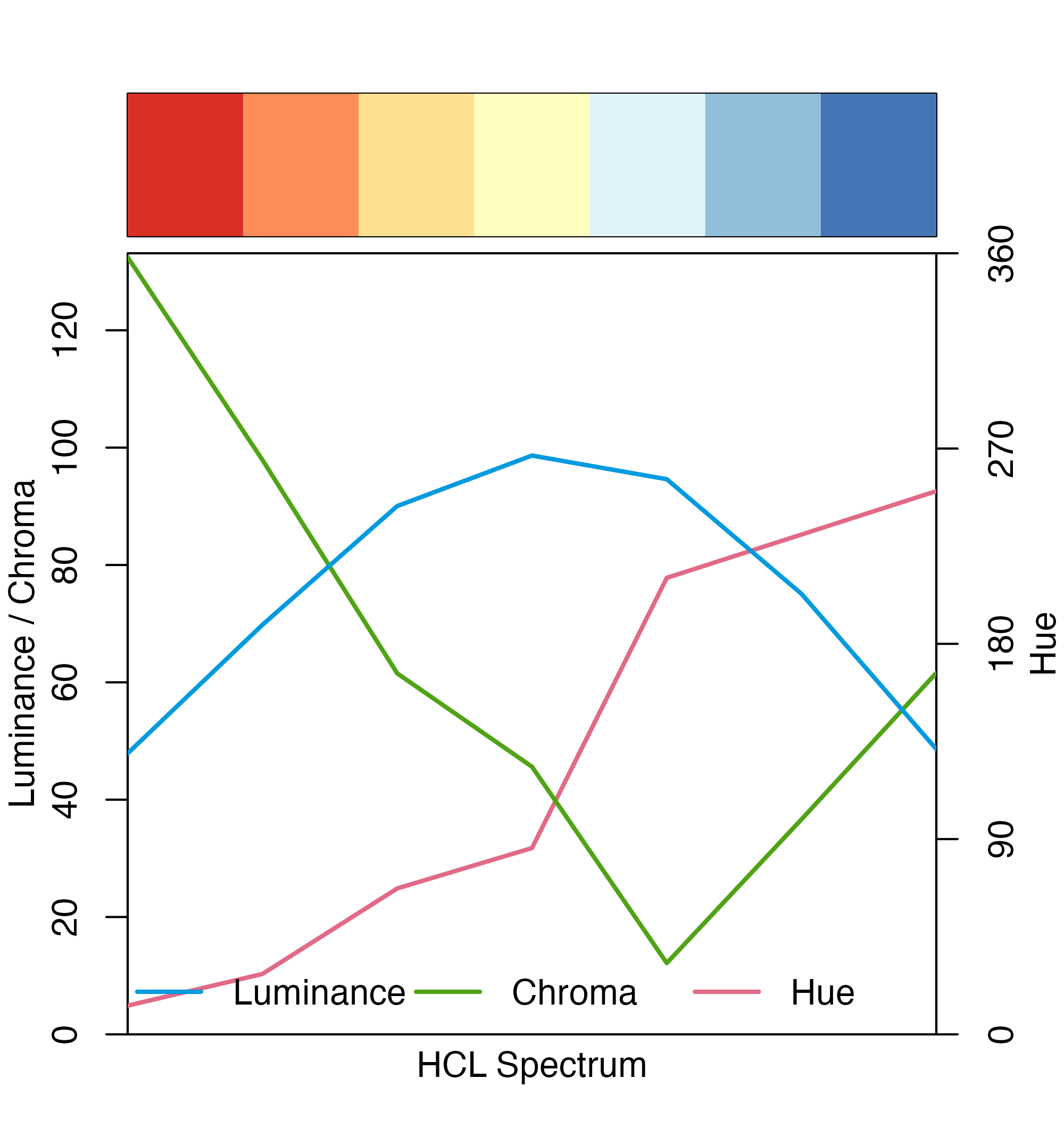
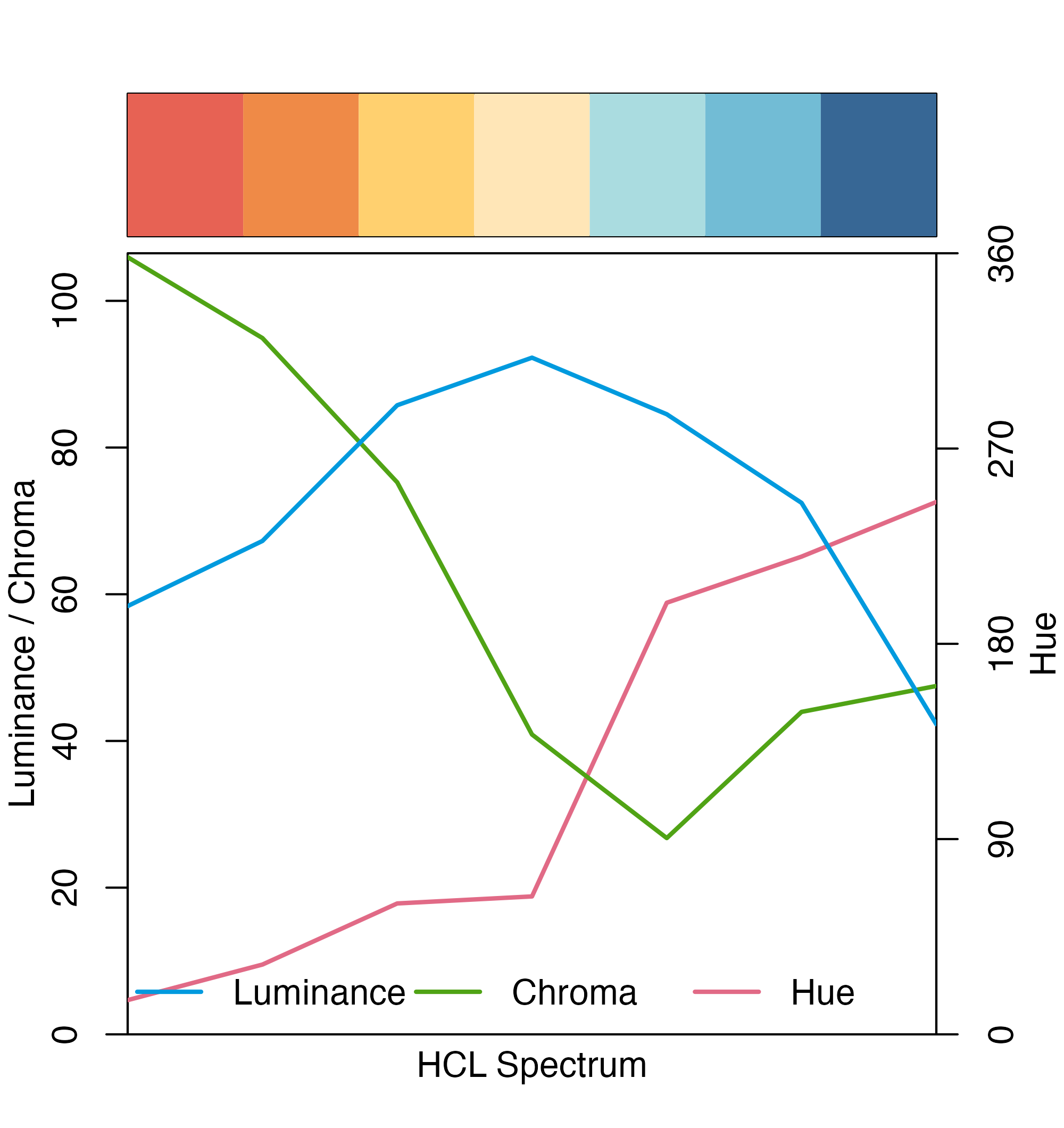
Evaluate HCL Space
Color Tools
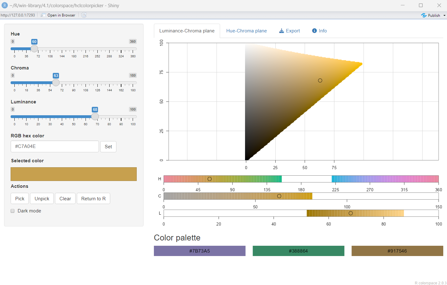
Color Tools

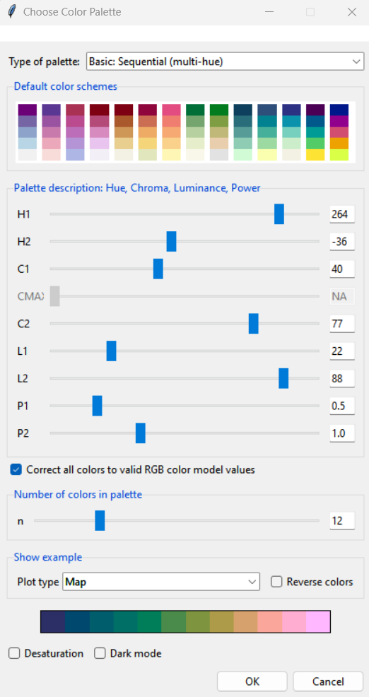
Color Palette Tools
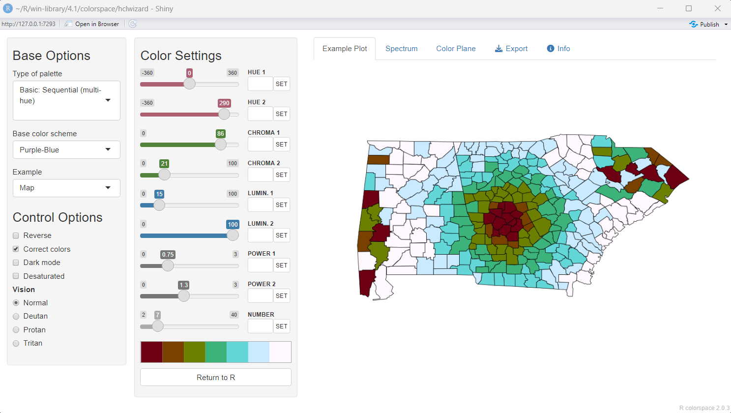
Color Palette Tools
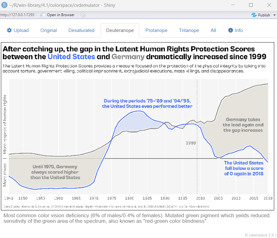
CVD Tool
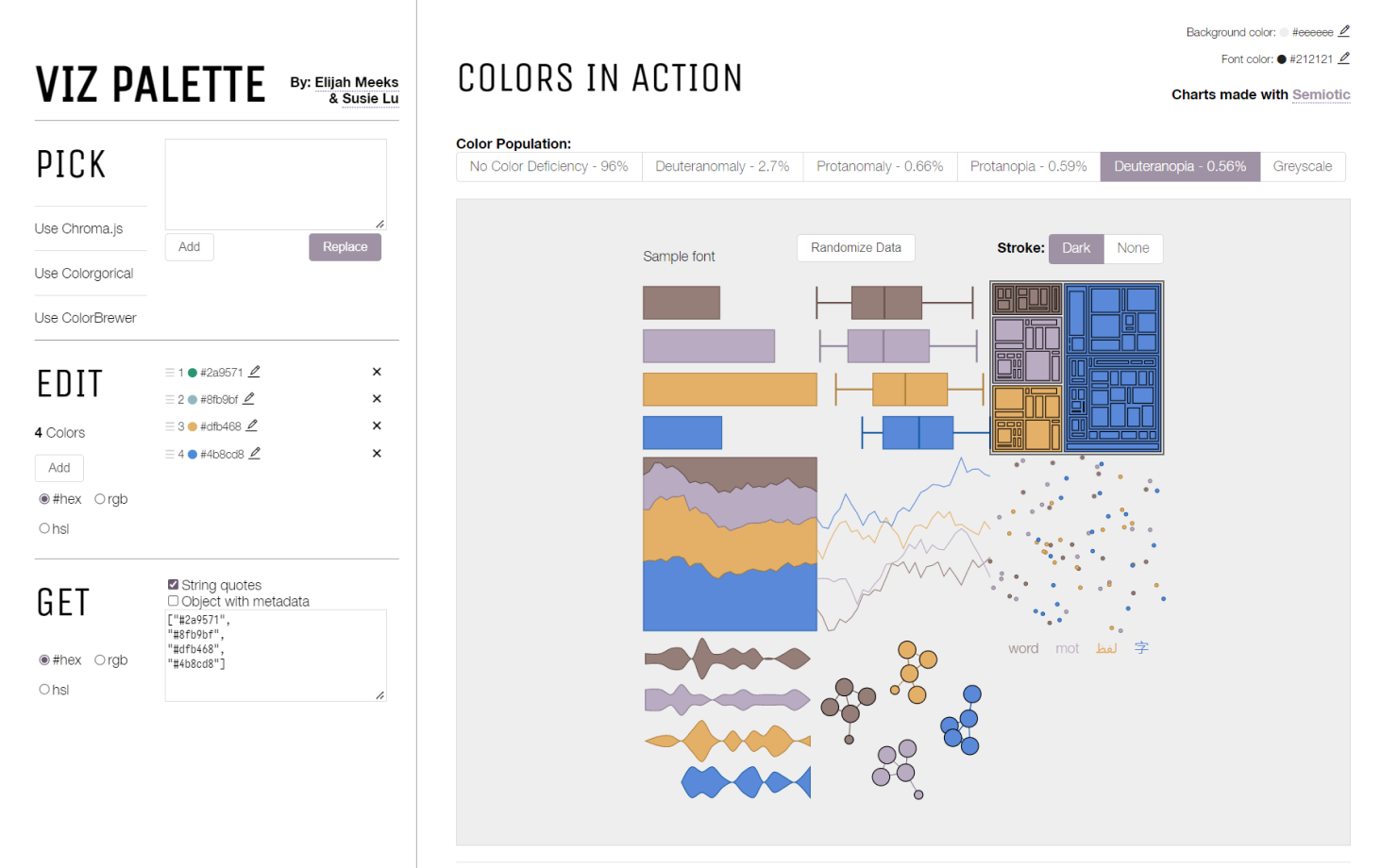
Viz Palette Tool
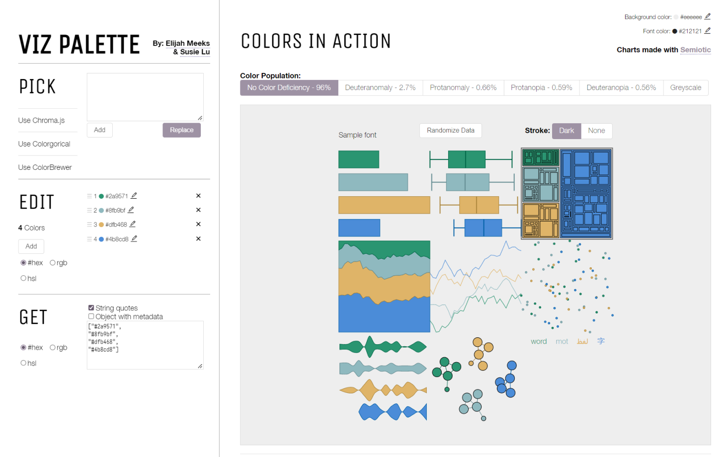
Viz Palette
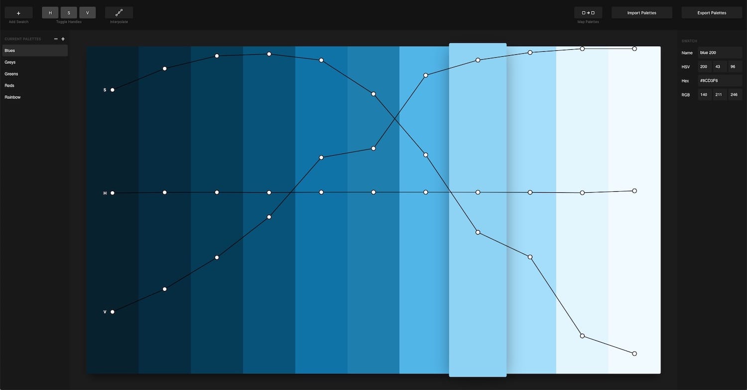
Palettte App
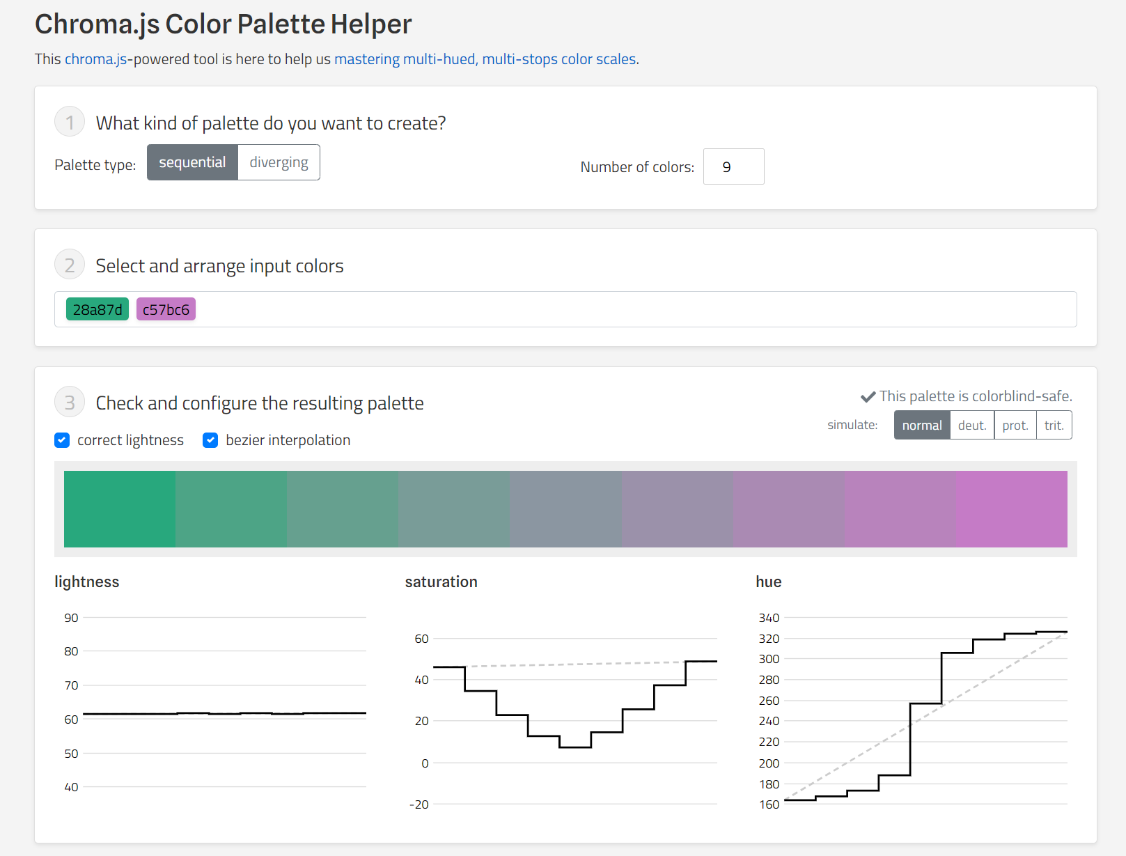
Chroma.js